Chapter 8: Counterfactuals: Mining Worlds That Could Have Been

Had Cleopatra's nose been shorter, the whole face of the world would have changed.

-BLAISE PASCAL (1669)

AS we prepare to move up to the top rung of the Ladder of Causation, let's recapitulate what we have learned from the second rung. We have seen several ways to ascertain the effect of an intervention in various settings and under a variety of conditions. In Chapter 4, we discussed randomized controlled trials, the widely cited 'gold standard' for medical trials. We have also seen methods that are suitable for observational studies, in which the treatment and control groups are not assigned at random. If we can measure variables that block all the back-door paths, we can use the back-door adjustment formula to obtain the needed effect. If we can find a front-door path that is 'shielded' from confounders, we can use front-door adjustment. If we are willing to live with the assumption of linearity or monotonicity, we can use instrumental variables (assuming that an appropriate variable can be found in the diagram or created by an experiment). And truly adventurous researchers can plot other routes to the top of Mount Intervention using the do -calculus or its algorithmic version.

In all these endeavors, we have dealt with effects on a population or a typical individual selected from a study population (the average causal effect). But so far we are missing the ability to talk about personalized causation at

the level of particular events or individuals. It's one thing to say, 'Smoking causes cancer,' but another to say that my uncle Joe, who smoked a pack a day for thirty years, would have been alive had he not smoked. The difference is both obvious and profound: none of the people who, like Uncle Joe, smoked for thirty years and died can ever be observed in the alternate world where they did not smoke for thirty years.

Responsibility and blame, regret and credit: these concepts are the currency of a causal mind. To make any sense of them, we must be able to compare what did happen with what would have happened under some alternative hypothesis. As argued in Chapter 1, our ability to conceive of alternative, nonexistent worlds separated us from our protohuman ancestors and indeed from any other creature on the planet. Every other creature can see what is. Our gift, which may sometimes be a curse, is that we can see what might have been.

This chapter shows how to use observational and experimental data to extract information about counterfactual scenarios. It explains how to represent individual-level causes in the context of a causal diagram, a task that will force us to explain some nuts and bolts of causal diagrams that we have not talked about yet. I also discuss a highly related concept called 'potential outcomes,' or the Neyman-Rubin causal model, initially proposed in the 1920s by Jerzy Neyman, a Polish statistician who later became a professor at Berkeley. But only after Donald Rubin began writing about potential outcomes in the mid-1970s did this approach to causal analysis really begin to flourish.

I will show how counterfactuals emerge naturally in the framework developed over the last several chapters-Sewall Wright's path diagrams and their extension to structural causal models (SCMs). We got a good taste of this in Chapter 1, in the example of the firing squad, which showed how to answer counterfactual questions such as 'Would the prisoner be alive if rifleman A had not shot?' I will compare how counterfactuals are defined in the Neyman-Rubin paradigm and in SCMs, where they enjoy the benefit of causal diagrams. Rubin has steadfastly maintained over the years that diagrams serve no useful purpose. So we will examine how students of the Rubin causal model must navigate causal problems blindfolded, lacking a facility to represent causal knowledge or to derive its testable implications.

Finally, we will look at two applications where counterfactual reasoning is essential. For decades or even centuries, lawyers have used a relatively straightforward test of a defendant's culpability called 'but-for causation': the

injury would not have occurred but for the defendant's action. We will see how the language of counterfactuals can capture this elusive notion and how to estimate the probability that a defendant is culpable.

Next, I will discuss the application of counterfactuals to climate change. Until recently, climate scientists have found it very difficult and awkward to answer questions like 'Did global warming cause this storm [or this heat wave, or this drought]?' The conventional answer has been that individual weather events cannot be attributed to global climate change. Yet this answer seems rather evasive and may even contribute to public indifference about climate change.

Counterfactual analysis allows climate scientists to make much more precise and definite statements than before. It requires, however, a slight addition to our everyday vocabulary. It will be helpful to distinguish three different kinds of causation: necessary causation, sufficient causation, and necessary-and-sufficient causation. (Necessary causation is the same as butfor causation.) Using these words, a climate scientist can say, 'There is a 90 percent probability that man-made climate change was a necessary cause of this heat wave,' or 'There is an 80 percent probability that climate change will be sufficient to produce a heat wave this strong at least once every 50 years.' The first sentence has to do with attribution: Who was responsible for the unusual heat? The second has to do with policy. It says that we had better prepare for such heat waves because they are likely to occur sooner or later. Either of these statements is more informative than shrugging our shoulders and saying nothing about the causes of individual weather events.

FROM THUCYDIDES AND ABRAHAM TO HUME AND LEWIS

Given that counterfactual reasoning is part of the mental apparatus that makes us human, it is not surprising that we can find counterfactual statements as far back as we want to go in human history. For example, in Thucydides's History of the Peloponnesian War , the ancient Greek historian, often described as the pioneer of a 'scientific' approach to history, describes a tsunami that occurred in 426 BC:

About the same time that these earthquakes were so common, the sea at Orobiae, in Euboea, retiring from the then line of coast, returned in a huge wave and invaded a great part of the town, and retreated leaving some of it still under water; so that what was once land is now sea;

such of the inhabitants perishing as could not run up to the higher ground in time.… The cause, in my opinion, of this phenomenon must be sought in the earthquake. At the point where its shock has been the most violent the sea is driven back, and suddenly recoiling with redoubled force, causes the inundation. Without an earthquake I do not see how such an accident could happen.

This is a truly remarkable passage when you consider the era in which it was written. First, the precision of Thucydides's observations would do credit to any modern scientist, and all the more so because he was working in an era when there were no satellites, no video cameras, no 24/7 news organizations broadcasting images of the disaster as it unfolded. Second, he was writing at a time in human history when natural disasters were ordinarily ascribed to the will of the gods. His predecessor Homer or his contemporary Herodotus would undoubtedly have attributed this event to the wrath of Poseidon or some other deity. Yet Thucydides proposes a causal model without any supernatural processes: the earthquake drives back the sea, which recoils and inundates the land. The last sentence of the quote is especially interesting because it expresses the notion of necessary or but-for causation: but for the earthquake, the tsunami could not have occurred. This counterfactual judgment promotes the earthquake from a mere antecedent of the tsunami to an actual cause.

Another fascinating and revealing instance of counterfactual reasoning occurs in the book of Genesis in the Bible. Abraham is talking with God about the latter's intention to destroy the cities of Sodom and Gomorrah as retribution for their evil ways.

And Abraham drew near, and said, Wilt thou really destroy the righteous with the wicked?

Suppose there be fifty righteous within the city: wilt thou also destroy and not spare the place for the sake of the fifty righteous that are therein?…

And the Lord said, If I find in Sodom fifty righteous within the city, then I will spare all the place for their sakes.

But the story does not end there. Abraham is not satisfied and asks the Lord, what if there are only forty-five righteous men? Or forty? Or thirty? Or twenty? Or even ten? Each time he receives an affirmative answer, and God ultimately assures him that he will spare Sodom even for the sake of ten righteous men, if he can find that many.

What is Abraham trying to accomplish with this haggling and bargaining? Surely he does not doubt God's ability to count. And of course, Abraham knows that God knows how many righteous men live in Sodom. He is, after all, omniscient.

Knowing Abraham's obedience and devotion, it is hard to believe that the questions are meant to convince the Lord to change his mind. Instead, they are meant for Abraham's own comprehension. He is reasoning just as a modern scientist would, trying to understand the laws that govern collective punishment. What level of wickedness is sufficient to warrant destruction? Would thirty righteous men be enough to save a city? Twenty? We do not have a complete causal model without such information. A modern scientist might call it a dose-response curve or a threshold effect.

While Thucydides and Abraham probed counterfactuals through individual cases, the Greek philosopher Aristotle investigated more generic aspects of causation. In his typically systematic style, Aristotle set up a whole taxonomy of causation, including 'material causes,' 'formal causes,' 'efficient causes,' and 'final causes.' For example, the material cause of the shape of a statue is the bronze from which it is cast and its properties; we could not make the same statue out of Silly Putty. However, Aristotle nowhere makes a statement about causation as a counterfactual, so his ingenious classification lacks the simple clarity of Thucydides's account of the cause of the tsunami.

To find a philosopher who placed counterfactuals at the heart of causality, we have to move ahead to David Hume, the Scottish philosopher and contemporary of Thomas Bayes. Hume rejected Aristotle's classification scheme and insisted on a single definition of causation. But he found this definition quite elusive and was in fact torn between two different definitions. Later these would turn into two incompatible ideologies, which ironically could both cite Hume as their source!

In his Treatise of Human Nature (Figure 8.1), Hume denies that any two objects have innate qualities or 'powers' that make one a cause and the other an effect. In his view, the cause-effect relationship is entirely a product of our own memory and experience. 'Thus we remember to have seen that species of object we call flame , and to have felt that species of sensation we call heat ,' he writes. 'We likewise call to mind their constant conjunction in all past instances. Without any further ceremony, we call the one cause and the other effect , and infer the existence of the one from the other.' This is now known as the 'regularity' definition of causation.

The passage is breathtaking in its chutzpah. Hume is cutting off the second and third rungs of the Ladder of Causation and saying that the first rung, observation, is all that we need. Once we observe flame and heat together a sufficient number of times (and note that flame has temporal precedence), we agree to call flame the cause of heat. Like most twentieth-century statisticians, Hume in 1739 seems happy to consider causation as merely a species of correlation.

A

T R E A T I $ E 0 F

Human Nature :

B E I N G

An ATTEMPT to introduce the ex perimental Method of Reafoning

1 N T 0

MORAL SUBJECTS

Rara temporum felicitas, ubi fentire, quæ velis ; 6 quæ TACIT.

Vo L.

0 F TH E

U NDER S T A NDI N G.

L0 N D 0 N:

near Hart,

MDCC XXXIX.

156 A Treatife %f Human Nature.

room

advancing we have infenfibly difcover'd a new relation betwixt caufe and

'TIs therefore by ExPE RIENCE only, that wC can infer the exiftence of from that of another. The of We remember to had frequent inftances of the exiftence of one fpecies of objects ; and allo that the individuals of another {pecies of objects have always attended and have exifted in order of contiguity aud fuccefion with regard to them Thus we remember to have feen that fpecies of objeet we call fame, and to have felt that {pecies of fenfation we call beat. We likewile call to mind their conftant conjuncion in all inftances. Without any farther ceremony, we call the one caufe and the other efe&t , and infer the exiftence of the one from that of the other. we learn fects, both the caules and effects have been perceiv'd by the fenfes; and are remember'd : But in all wherein we reafon concernthem, there is only one the other is fupply'd conformity to our experience. one ject nature have remember, them, regular paf cafes, ing perceiv'd paf

FIGURE 8.1. Hume's 'regularity' definition of cause and effect, proposed in 1739.

And yet Hume, to his credit, did not remain satisfied with this definition. Nine years later, in An Enquiry Concerning Human Understanding , he wrote something quite different: 'We may define a cause to be an object followed by another, and where all the objects, similar to the first, are followed by objects similar to the second . Or, in other words, where, if the first object had not been, the second never had existed ' (emphasis in the original). The first sentence, the version where A is consistently observed together with B , simply repeats the regularity definition. But by 1748, he seems to have some misgivings and finds it in need of some repair. As authorized Whiggish historians, we can understand why. According to his earlier definition, the rooster's crow would cause sunrise. To patch over this difficulty, he adds a second definition that he never even hinted at in his earlier book, a counterfactual definition: 'if the first object had not been, the second had

probabi -

never existed.'

Note that the second definition is exactly the one that Thucydides used when he discussed the tsunami at Orobiae. The counterfactual definition also explains why we do not consider the rooster's crow a cause of sunrise. We know that if the rooster was sick one day, or capriciously refused to crow, the sun would rise anyway.

Although Hume tries to pass these two definitions off as one, by means of his innocent interjection 'in other words,' the second version is completely different from the first. It explicitly invokes a counterfactual, so it lies on the third rung of the Ladder of Causation. Whereas regularities can be observed, counterfactuals can only be imagined.

It is worth thinking for a moment about why Hume chooses to define causes in terms of counterfactuals, rather than the other way around. Definitions are intended to reduce a more complicated concept to a simpler one. Hume surmises that his readers will understand the statement 'if the first object had not been, the second had never existed' with less ambiguity than they will understand 'the first object caused the second.' He is absolutely right. The latter statement invites all sorts of fruitless metaphysical speculation about what quality or power inherent in the first object brings about the second one. The former statement merely asks us to perform a simple mental test: imagine a world without the earthquake and ask whether it also contains a tsunami. We have been making judgments like this since we were children, and the human species has been making them since Thucydides (and probably long before).

Nevertheless, philosophers ignored Hume's second definition for most of the nineteenth and twentieth centuries. Counterfactual statements, the 'would haves,' have always appeared too squishy and uncertain to satisfy academics. Instead, philosophers tried to rescue Hume's first definition through the theory of probabilistic causation, as discussed in Chapter 1.

One philosopher who defied convention, David Lewis, called in his 1973 book Counterfactuals for abandoning the regularity account altogether and for interpreting ' A has caused B ' as ' B would not have occurred if not for A .' Lewis asked, 'Why not take counterfactuals at face value: as statements about possible alternatives to the actual situation?'

Like Hume, Lewis was evidently impressed by the fact that humans make counterfactual judgments without much ado, swiftly, comfortably, and consistently. We can assign them truth values and probabilities with no less

confidence than we do for factual statements. In his view, we do this by envisioning 'possible worlds' in which the counterfactual statements are true.

When we say, 'Joe's headache would have gone away if he had taken aspirin,' we are saying (according to Lewis) that there are other possible worlds in which Joe did take an aspirin and his headache went away. Lewis argued that we evaluate counterfactuals by comparing our world, where he did not take aspirin, to the most similar world in which he did take an aspirin. Upon finding no headache in that world, we declare the counterfactual statement to be true. 'Most similar' is key. There may be some 'possible worlds' in which his headache did not go away-for example, a world in which he took the aspirin and then bumped his head on the bathroom door. But that world contains an extra, adventitious circumstance. Among all possible worlds in which Joe took aspirin, the one most similar to ours would be one not where he bumped his head but where his headache is gone.

Many of Lewis's critics pounced on the extravagance of his claims for the literal existence of many other possible worlds. 'Mr. Lewis was once dubbed a 'mad-dog modal realist' for his idea that any logically possible world you can think of actually exists,' said his New York Times obituary in 2001. 'He believed, for instance, that there was a world with talking donkeys.'

But I think that his critics (and perhaps Lewis himself) missed the most important point. We do not need to argue about whether such worlds exist as physical or even metaphysical entities. If we aim to explain what people mean by saying ' A causes B ,' we need only postulate that people are capable of generating alternative worlds in their heads, judging which world is 'closer' to ours and, most importantly, doing it coherently so as to form a consensus. Surely we could not communicate about counterfactuals if one person's 'closer' was another person's 'farther.' In this view, Lewis's appeal 'Why not take counterfactuals at face value?' called not for metaphysics but for attention to the amazing uniformity of the architecture of the human mind.

As a licensed Whiggish philosopher, I can explain this consistency quite well: it stems from the fact that we experience the same world and share the same mental model of its causal structure. We talked about this all the way back in Chapter 1. Our shared mental models bind us together into communities. We can therefore judge closeness not by some metaphysical notion of 'similarity' but by how much we must take apart and perturb our shared model before it satisfies a given hypothetical condition that is contrary to fact (Joe not taking aspirin).

In structural models we do a very similar thing, albeit embellished with

more mathematical detail. We evaluate expressions like 'had X been x ' in the same way that we handled interventions do X ( = x ), by deleting arrows in a causal diagram or equations in a structural model. We can describe this as making the minimal alteration to a causal diagram needed to ensure that X equals x . In this respect, structural counterfactuals are compatible with Lewis's idea of the most similar possible world.

Structural models also offer a resolution of a puzzle Lewis kept silent about: How do humans represent 'possible worlds' in their minds and compute the closest one, when the number of possibilities is far beyond the capacity of the human brain? Computer scientists call this the 'representation problem.' We must have some extremely economical code to manage that many worlds. Could structural models, in some shape or form, be the actual shortcut that we use? I think it is very likely, for two reasons. First, structural causal models are a shortcut that works, and there aren't any competitors around with that miraculous property. Second, they were modeled on Bayesian networks, which in turn were modeled on David Rumelhart's description of message passing in the brain. It is not too much of a stretch to think that 40,000 years ago, humans co-opted the machinery in their brain that already existed for pattern recognition and started to use it for causal reasoning.

Philosophers tend to leave it to psychologists to make statements about how the mind does things, which explains why the questions above were not addressed until quite recently. However, artificial intelligence (AI) researchers could not wait. They aimed to build robots that could communicate with humans about alternate scenarios, credit and blame, responsibility and regret. These are all counterfactual notions that AI researchers had to mechanize before they had the slightest chance of achieving what they call 'strong AI'humanlike intelligence.

With these motivations I entered counterfactual analysis in 1994 (with my student Alex Balke). Not surprisingly, the algorithmization of counterfactuals made a bigger splash in artificial intelligence and cognitive science than in philosophy. Philosophers tended to view structural models as merely one of many possible implementations of Lewis's possible-worlds logic. I dare to suggest that they are much more than that. Logic void of representation is metaphysics. Causal diagrams, with their simple rules of following and erasing arrows, must be close to the way that our brains represent counterfactuals.

This assertion must remain unproven for the time being, but the upshot of

the long story is that counterfactuals have ceased to be mystical. We understand how humans manage them, and we are ready to equip robots with similar capabilities to the ones our ancestors acquired 40,000 years ago.

POTENTIAL OUTCOMES, STRUCTURAL EQUATIONS, AND THE ALGORITHMIZATION OF COUNTERFACTUALS

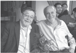
Just a year after the release of Lewis's book, and independently of it, Donald Rubin (Figure 8.2) began writing a series of papers that introduced potential outcomes as a language for asking causal questions. Rubin, at that time a statistician for the Educational Testing Service, single-handedly broke the silence about causality that had persisted in statistics for seventy-five years and legitimized the concept of counterfactuals in the eyes of many health scientists. It is impossible to overstate the importance of this development. It provided researchers with a flexible language to express almost every causal question they might wish to ask, at both the population and individual levels.

FIGURE 8.2. Donald Rubin (right) with the author in 2014. ( Source: Photo courtesy of Grace Hyun Kim.)

In the Rubin causal model, a potential outcome of a variable Y is simply 'the value that Y would have taken for individual u , had X been assigned the value x .' That's a lot of words, so it's often convenient to write this quantity more compactly as Y X = x ( u ). Often we abbreviate this further as Y x ( u ) if it is apparent from the context what variable is being set to the value x .

To appreciate how audacious this notation is, you have to step back from the symbols and think about the assumptions they embody. By writing down the symbol Y x , Rubin asserted that Y definitely would have taken some value if X had been x , and this has just as much objective reality as the value Y actually did take. If you don't buy this assumption (and I'm pretty sure Heisenberg wouldn't), you can't use potential outcomes. Also, note that the potential outcome, or counterfactual, is defined at the level of an individual, not a population.

The very first scientific appearance of a potential outcome came in the master's thesis of Jerzy Neyman, written in 1923. Neyman, a descendant of Polish nobility, had grown up in exile in Russia and did not set foot in his native land until 1921, when he was twenty-seven years old. He had received a very strong mathematical education in Russia and would have liked to continue research in pure mathematics, but it was easier for him to find employment as a statistician. Much like R. A. Fisher in England, he did his first statistical research at an agricultural institute, a job for which he was hugely overqualified. Not only was he the only statistician in the institute, but he was really the only person in the country thinking about statistics as a discipline.

Neyman's first mention of potential outcomes came in the context of an agricultural experiment, where the subscript notation represents the 'unknown potential yield of the ith variety [of a given seed] on the respective plot.' The thesis remained unknown and untranslated into English until 1990. However, Neyman himself did not remain unknown. He arranged to spend a year at Karl Pearson's statistical laboratory at University College London, where he made friends with Pearson's son Egon. The two kept in touch for the next seven years, and their collaboration paid great dividends: the NeymanPearson approach to statistical hypothesis testing was a milestone that every beginning statistics student learns about.

In 1933, Karl Pearson's long autocratic leadership finally came to an end with his retirement, and Egon was his logical successor-or would have been, if not for the singular problem of R. A. Fisher, by then the most famous statistician in England. The university came up with a unique and disastrous solution, dividing Pearson's position into a chair of statistics (Egon Pearson) and a chair of eugenics (Fisher). Egon wasted no time hiring his Polish friend. Neyman arrived in 1934 and almost immediately locked horns with Fisher.

Fisher was already spoiling for a fight. He knew he was the world's leading statistician and had practically invented large parts of the subject, yet was forbidden from teaching in the statistics department. Relations were extraordinarily tense. 'The Common Room was carefully shared,' writes Constance Reid in her biography of Neyman. 'Pearson's group had tea at 4; and at 4:30, when they were safely out of the way, Fisher and his group trooped in.'

In 1935, Neyman gave a lecture at the Royal Statistical Society titled 'Statistical Problems in Agricultural Experimentation,' in which he called into question some of Fisher's own methods and also, incidentally, discussed

the idea of potential outcomes. After Neyman was done, Fisher stood up and told the society that 'he had hoped that Dr. Neyman's paper would be on a subject with which the author was fully acquainted.'

'[Neyman had] asserted that Fisher was wrong,' wrote Oscar Kempthorne years later about the incident. 'This was an unforgivable offense-Fisher was never wrong and indeed the suggestion that he might be was treated by him as a deadly assault. Anyone who did not accept Fisher's writing as the Godgiven truth was at best stupid and at worst evil.' Neyman and Pearson saw the extent of Fisher's fury a few days later, when they went to the department in the evening and found Neyman's wooden models, with which he had illustrated his lecture, strewn all over the floor. They concluded that only Fisher could have been responsible for the wreckage.

While Fisher's fit of rage may seem amusing now, his attitude did have serious consequences. Of course he could not swallow his pride and use Neyman's potential outcome notation, even though it would have helped him later with problems of mediation. The lack of potential outcome vocabulary led him and many other people into the so-called Mediation Fallacy, which we will discuss in Chapter 9.

At this point some readers might still find the concept of counterfactuals somewhat mystical, so I'd like to show how some of Rubin's followers would infer potential outcomes and contrast this model-free approach with the structural causal model approach.

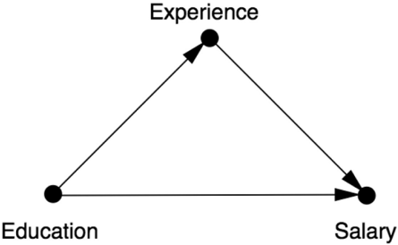
Suppose that we are looking at a certain firm to see whether education or years of experience is a more important factor in determining an employee's salary. We have collected some data on the existing salaries at this firm, reproduced in Table 8.1. We're letting EX represent years of experience, ED represent education, and S represent salary. We're also assuming, for simplicity, just three levels of education: 0 = high school degree, 1 = college degree, 2 = graduate degree. Thus S ED = 0 ( u ), or S 0 ( u ), represents the salary of individual u if u were a high school graduate but not a college graduate, and S 1 ( u ) represents u 's salary if u were a college graduate. A typical counterfactual question we might want to ask is, 'What would Alice's salary be if she had a college degree?' In other words, what is S 1 (Alice)?

The first thing to notice about Table 8.1 is all the missing data, indicated by question marks. We can never observe more than one potential outcome in the same individual. Although obvious, nevertheless this statement is important. Statistician Paul Holland once called it the 'fundamental problem of causal inference,' a name that has stuck. If we could only fill in the

question marks, we could answer all our causal questions.

I have never agreed with Holland's characterization of the missing values in Table 8.1 as a 'fundamental problem,' perhaps because I have rarely described causal problems in terms of a table. But more fundamentally, viewing causal inference as a missing-data problem can be terribly misleading, as we will soon see. Observe that, aside from the decorative headings of the last three columns, Table 8.1 is totally devoid of causal information about ED EX , , and S -for example, whether education affects salary or the other way around. Worse yet, it does not allow us to represent such information when available. But for statisticians who perceive the 'fundamental problem' to be missing data, such a table appears to present endless opportunities. Indeed, if we look at S 0 , S 1 , and S 2 not as potential outcomes but as ordinary variables, we have dozens of interpolation techniques to fill in the blanks or, as statisticians would say, 'impute the missing data,' in some optimal way.

TABLE 8.1. Fictitious data for potential outcomes example.

One common approach is matching. We look for pairs of individuals who are well matched in all variables except the one of interest and then fill in their rows to match each other. The clearest case here is that of Bert and Caroline, who match perfectly on experience. So we assume that Bert's salary, if he had a graduate degree, would be the same as Caroline's ($97,000), and Caroline's salary, if she had only an undergraduate degree, would be the same as Bert's ($92,500). Note that matching invokes the same idea as conditioning (or stratifying): we select for comparison groups that share an observed characteristic and use the comparison to infer characteristics that they do not seem to share.

It is hard to estimate Alice's salary this way because there is no good match for her in the data I have given. Nevertheless, statisticians have

developed techniques of considerable subtlety to impute missing data from approximate matches, and Rubin has been a pioneer of this approach. Unfortunately, even the most gifted matchmaker in the world cannot turn data into potential outcomes, not even approximately. I will show below that the correct answer depends critically on whether education affects experience or the other way around, information nowhere to be found in the table.

A second possible method is linear regression (not to be conflated with structural equations). In this approach we pretend that the data came from some unknown random source and use standard statistical methods to find the line (or, in this case, plane) that best fits the data. The output of such an approach might be an equation that looks like this:

$$S = $65,000 + 2,500 × EX + 5,000 × ED (8.1)$$ Equation 8.1 tells us that (on average) the base salary of an employee with no experience and only a high school diploma is $65,000. For each year of experience, the salary increases by $2,500, and for each additional educational degree (up to two), the salary increases by $5,000. Accordingly, a regression analyst would claim, our estimate of Alice's salary, if she had a college degree, is $65,000 + $2,500 × 6 + $5,000 × 1 = $85,000.

The ease and familiarity of such imputation techniques explain why Rubin's conception of causal inference as a missing-data problem has enjoyed broad popularity. Alas, as innocuous as these interpolation methods appear, they are fundamentally flawed. They are data driven, not model driven. All the missing data are filled in by examining other values in the table. As we have learned from the Ladder of Causation, any such method is doomed to start with; no methods based only on data (rung one) can answer counterfactual questions (rung three).

Before contrasting these methods with the structural causal model approach, let us examine intuitively what goes wrong with model-blind imputation. In particular, let us explain why Bert and Caroline, who match perfectly in experience, may in fact be quite incomparable when it comes to comparing their potential outcomes. More surprising, a reasonable causal story (fitting Table 8.1) would show that the best match for Caroline for Salary would be someone who does not match her on Experience.

The first key point to realize is that Experience is likely to depend on Education. After all, those employees who got an extra educational degree took four years of their lives to do so. Thus, if Caroline had only one degree of education (like Bert), she would have been able to use that extra time to

gain more experience compared to what she now has. This would have given her equal education to and greater experience than Bert. We can thus conclude that S 1 (Caroline) > S 1 (Bert), contrary to what naive matching would predict. We see that, once we have a causal story in which Education affects Experience, it is inevitable that 'matching' on Experience will create a mismatch on potential Salary.

Ironically, equal Experience, which started out as an invitation for matching, has now turned into a loud warning against it. Table 8.1 will, of course, continue its silence about such dangers. For this reason I cannot share Holland's enthusiasm for casting causal inference as a missing-data problem. Quite the contrary. Recent work of Karthika Mohan, a former student of mine, reveals that even standard problems of missing data require causal modeling for their solution.

Now let's see how a structural causal model would treat the same data. First, before we even look at the data, we draw a causal diagram (Figure 8.3). The diagram encodes the causal story behind the data, according to which Experience listens to Education and Salary listens to both. In fact, we can already tell something very important just by looking at the diagram. If our model were wrong and EX were a cause of ED , rather than vice versa, then Experience would be a confounder, and matching employees with similar experience would be completely appropriate. With ED as the cause of EX , Experience is a mediator. As you surely know by now, mistaking a mediator for a confounder is one of the deadliest sins in causal inference and may lead to the most outrageous errors. The latter invites adjustment; the former forbids it.

FIGURE 8.3. Causal diagram for the effect of education ( ED ) and experience ( EX ) on salary ( S ).

So far in this book, I have used a very informal word-'listening'-to express what I mean by the arrows in a causal diagram. But now it's time to put a little bit of mathematical meat on this concept, and this is in fact where

structural causal models differ from Bayesian networks or regression models. When I say that Salary listens to Education and Experience, I mean that it is a mathematical function of those variables: S = f S ( EX , ED ). But we need to allow for individual variations, so we extend this function to read S = f S ( EX , ED U , S ), where U S stands for 'unobserved variables that affect salary.' We know these variables exist (e.g., Alice is a friend of the company's president), but they are too diverse and too numerous to incorporate explicitly into our model.

Let's see how this would play out in our education/experience/salary example, assuming linear functions throughout. We can use the same statistical methods as before to find the best-fitting linear equation. The result would look just like Equation 8.1 with one small difference:

$$S = $65,000 + 2,500 × EX + 5,000 × ED + U S (8.2)$$ However, the formal similarity between Equations 8.1 and 8.2 is profoundly deceptive; their interpretations differ like night and day. The fact that we chose to regress S on ED and EX in Equation 8.1 in no way implies that S listens to ED and EX in the real world. That choice was purely ours, and nothing in the data would prevent us from regressing EX on ED and S or following any other order. (Remember Francis Galton's discovery in Chapter 2 that regressions are cause blind.) We lose this freedom once we proclaim an equation to be 'structural.' In other words, the author of Equation 8.2 must commit to writing equations that mirror his belief about who listens to whom in the world. In our case, he believes that S truly listens to EX and ED . More importantly, the absence of an equation ED = f ED ( EX S U , , ED ) from the model means that ED is believed to be oblivious to changes in EX or S . This difference in commitment gives structural equations the power to support counterfactuals, a power denied to regression equations.

In compliance with Figure 8.3, we must also have a structural equation for EX , but now we will force the coefficient of S to zero, to reflect the absence of an arrow from S to EX . Once we estimate the coefficients from the data, the equation might look something like this:

$$EX = 10-4 × ED + U EX (8.3)$$ This equation says that the average experience for people with no advanced degrees is ten years, and each degree of education (up to two) decreases EX by four years on average. Again, note the key difference between structural and regression equations: variable S does not enter into Equation 8.3, despite the fact that S and EX are likely to be highly correlated. This reflects the

analyst's belief that the experience EX acquired by any individual is totally unaffected by his current salary.

Now let's demonstrate how to derive counterfactuals from a structural model. To estimate Alice's salary if she had a college education, we perform three steps:

• 1. (Abduction) Use the data about Alice and about the other employees to estimate Alice's idiosyncratic factors, U S (Alice) and U EX (Alice).
• 2. (Action) Use the do -operator to change the model to reflect the counterfactual assumption being made, in this case that she has a college degree: ED (Alice) = 1.
• 3. (Prediction) Calculate Alice's new salary using the modified model and the updated information about the exogenous variables U S (Alice), U EX (Alice), and ED (Alice). This newly calculated salary is equal to S ED = 1 (Alice).

For step 1, we observe from the data that EX (Alice) = 6 and ED (Alice) = 0. We substitute these values into Equations 8.2 and 8.3. The equations then tell us Alice's idiosyncratic factors: U S (Alice) = $1,000 and U EX (Alice) = -4. This represents everything that is unique, special, and wonderful about Alice. Whatever that is, it adds $1,000 to her predicted salary.

Step 2 tells us to use the do -operator to erase the arrows pointing to the variable that is being set to a counterfactual value (Education) and set Alice's Education to a college degree (Education = 1). In this example, Step 2 is trivial, because there are no arrows pointing to Education and hence no arrows to erase. In more complicated models, though, this step of erasing the arrows cannot be left out, because it affects the computation in Step 3. Variables that might have affected the outcome through the intervened variable will no longer be allowed to do so.

Finally, Step 3 says to update the model to reflect the new information that U S = $1,000, U EX = -4, and ED = 1. First we use Equation 8.3 to recompute what Alice's Experience would be if she had gone to college: EX ED = 1 (Alice) = 10 - 4 - 4 = 2 years. Then we use Equation 8.2 to recompute her potential Salary:

S ED = 1 (Alice) = $65,000 + 2,500 × 2 + 5,000 × 1 + 1,000 = $76,000.

Our result, S 1 (Alice) = $76,000, is a valid estimate of Alice's would-be salary; that is, the two will coincide if the model assumptions are valid. Because this example entails a very simple causal model and very simple (linear) functions, the differences between it and the data-driven regression method may seem rather minor. But the minor differences on the surface reflect vast differences underneath. Whatever counterfactual (potential) outcome we obtain from the structural method follows logically from the assumptions displayed in the model, while the answer obtained by the datadriven method is as whimsical as spurious correlations because it leaves important modeling assumptions unaccounted for.

This example has forced us to go further into the 'nuts and bolts' of causal models than we have previously done in this book. But let me step back a little to celebrate and appreciate the miracle that came into being through Alice's example. Using a combination of data and model, we were able to predict the behavior of an individual (Alice) under totally hypothetical conditions. Of course, there is no such thing as a free lunch: we got these strong results because we made strong assumptions. In addition to asserting the causal relationships between the observed variables, we also assumed that the functional relationships were linear. But the linearity matters less here than knowing what those specific functions are. That enabled us to compute Alice's idiosyncrasies from her observed characteristics and update the model as required in the three-step procedure.

At the risk of adding a sober note to our celebration, I have to tell you that this functional information will not always be available to us in practice. In general, we call a model 'completely specified' if the functions behind the arrows are known and 'partially specified' otherwise. For instance, as in Bayesian networks, we may only know probabilistic relationships between parents and children in the graph. If the model is partially specified, we may not be able to estimate Alice's salary exactly; instead we may have to make a probability-interval statement, such as 'There is a 10 to 20 percent chance that her salary would be $76,000.' But even such probabilistic answers are good enough for many applications. Moreover, it is truly remarkable how much information we can extract from the causal diagram even when we have no information on the specific functions lying behind the arrows or only very general information, such as the 'monotonicity' assumption we encountered in the last chapter.

Steps 1 to 3 above can be summed up in what I call the 'first law of causal inference': Y x ( u ) = Y Mx ( u ). This is the same rule that we used in the firing

squad example in Chapter 1, except that the functions are different. The first law says that the potential outcome Y x ( u ) can be imputed by going to the model M x (with arrows into X deleted) and computing the outcome Y u ( ) there. All estimable quantities on rungs two and three of the Ladder of Causation follow from there. In short, the reduction of counterfactuals to an algorithm allows us to conquer as much territory from rung three as mathematics will permit-but, of course, not a bit more.

THE VIRTUE OF SEEING YOUR ASSUMPTIONS

The SCM method I have shown for computing counterfactuals is not the same method that Rubin would use. A major point of difference between us is the use of causal diagrams. They allow researchers to represent causal assumptions in terms that they can understand and then treat all counterfactuals as derived properties of their world model. The Rubin causal model treats counterfactuals as abstract mathematical objects that are managed by algebraic machinery but not derived from a model.

Deprived of a graphical facility, the user of the Rubin causal model is usually asked to accept three assumptions. The first one, called the 'stable unit treatment value assumption,' or SUTVA, is reasonably transparent. It says that each individual (or 'unit,' the preferred term of causal modelers) will have the same effect of treatment regardless of what treatment the other individuals (or 'units') receive. In many cases, barring epidemics and other collective interactions, this makes perfectly good sense. For example, assuming headache is not contagious, my response to aspirin will not depend on whether Joe receives aspirin.

The second assumption in Rubin's model, also benign, is called 'consistency.' It says that a person who took aspirin and recovered would also recover if given aspirin by experimental design. This reasonable assumption, which is a theorem in the SCM framework, says in effect that the experiment is free of placebo effects and other imperfections.

But the major assumption that potential outcome practitioners are invariably required to make is called 'ignorability.' It is more technical, but it's the crucial part of the transaction, for it is in essence the same thing as Jamie Robins and Sander Greenland's condition of exchangeability discussed in Chapter 4. Ignorability expresses this same requirement in terms of the potential outcome variable Y x . It requires that Y x be independent of the

treatment actually received, namely X , given the values of a certain set of (de)confounding variables Z . Before exploring its interpretation, we should acknowledge that any assumption expressed as conditional independence inherits a large body of familiar mathematical machinery developed by statisticians for ordinary (noncounterfactual) variables. For example, statisticians routinely use rules for deciding when one conditional independence follows from another. To Rubin's credit, he recognized the advantages of translating the causal notion of 'nonconfoundedness' into the syntax of probability theory, albeit on counterfactual variables. The ignorability assumption makes the Rubin causal model actually a model; Table 8.1 in itself is not a model because it contains no assumptions about the world.

Unfortunately, I have yet to find a single person who can explain what ignorability means in a language spoken by those who need to make this assumption or assess its plausibility in a given problem. Here is my best try. The assignment of patients to either treatment or control is ignorable if, within any stratum of the confounder Z , patients who would have one potential outcome, Y x = y , are just as likely to be in the treatment or control group as the patients who would have a different potential outcome, Y x = y '. This definition is perfectly legitimate for someone in possession of a probability function over counterfactuals. But how is a biologist or economist with only scientific knowledge for guidance supposed to assess whether this is true or not? More concretely, how is a scientist to assess whether ignorability holds in any of the examples discussed in this book?

To understand the difficulty, let us attempt to apply this explanation to our example. To determine if ED is ignorable (conditional on EX ), we are supposed to judge whether employees who would have one potential salary, say S 1 = s , are just as likely to have one level of education as the employees who would have a different potential salary, say S 1 = s '. If you think that this sounds circular, I can only agree with you! We want to determine Alice's potential salary, and even before we start-even before we get a hint about the answer-we are supposed to speculate on whether the result is dependent or independent of ED , in every stratum of EX . It is quite a cognitive nightmare.

As it turns out, ED in our example is not ignorable with respect to S , conditional on EX , and this is why the matching approach (setting Bert and Caroline equal) would yield the wrong answer for their potential salaries. In fact, their estimates should differ by an amount S 1 (Bert)S 1 (Caroline) =

$5,000. (The reader should be able to show this from the numbers in Table 8.1 and the three-step procedure.) I will now show that with the help of a causal diagram, a student could see immediately that ED is not ignorable and would not attempt matching here. Lacking a diagram, a student would be tempted to assume that ignorability holds by default and would fall into this trap. (This is not a speculation. I borrowed the idea for this example from an article in Harvard Law Review where the story was essentially the same as in Figure 8.3 and the author did use matching.)

Here is how we can use a causal diagram to test for (conditional) ignorability. To determine if X is ignorable relative to outcome Y , conditional on a set Z of matching variables, we need only test to see if Z blocks all the back-door paths between X and Y and no member of Z is a descendant of X . It is as simple as that! In our example, the proposed matching variable (Experience) blocks all the back-door paths (because there aren't any), but it fails the test because it is a descendant of Education. Therefore ED is not ignorable, and EX cannot be used for matching. No elaborate mental gymnastics are needed, just a look at a diagram. Never is a researcher required to mentally assess how likely a potential outcome is given one treatment or another.

Unfortunately, Rubin does not consider causal diagrams to 'aid the drawing of causal inferences.' Therefore, researchers who follow his advice will be deprived of this test for ignorability and will either have to perform formidable mental gymnastics to convince themselves that the assumption holds or else simply accept the assumption as a 'black box.' Indeed, a prominent potential outcome researcher, Marshall Joffe, wrote in 2010 that ignorability assumptions are usually made because they justify the use of available statistical methods, not because they are truly believed.

Closely related to transparency is the notion of testability, which has come up several times in this book. A model cast as a causal diagram can easily be tested for compatibility with the data, whereas a model cast in potential outcome language lacks this feature. The test goes like this: whenever all paths between X and Y in the diagram are blocked by a set of nodes Z , then in the data X and Y should be independent, conditional on Z . This is the d -separation property mentioned in Chapter 7, which allows us to reject a model whenever the independence fails to show up in the data. In contrast, if the same model is expressed in the language of potential outcomes (i.e., as a collection of ignorability statements), we lack the mathematical machinery to unveil the independencies that the model entails, and researchers are unable to subject the model to a test. It is hard to understand how potential outcome

researchers managed to live with this deficiency without rebelling. My only explanation is that they were kept away from graphical tools for so long that they forgot that causal models can and should be testable.

Now I must apply the same standards of transparency to myself and say a little bit more about the assumptions embodied in a structural causal model.

Remember the story of Abraham that I related earlier? Abraham's first response to the news of Sodom's imminent destruction was to look for a doseresponse relationship, or a response function, relating the wickedness of the city to its punishment. It was a sound scientific instinct, but I suspect few of us would have been calm enough to react that way.

The response function is the key ingredient that gives SCMs the power to handle counterfactuals. It is implicit in Rubin's potential outcome paradigm but a major point of difference between SCMs and Bayesian networks, including causal Bayesian networks. In a probabilistic Bayesian network, the arrows into Y mean that the probability of Y is governed by the conditional probability tables for Y , given observations of its parent variables. The same is true for causal Bayesian networks, except that the conditional probability tables specify the probability of Y given interventions on the parent variables. Both models specify probabilities for Y , not a specific value of Y . In a structural causal model, there are no conditional probability tables. The arrows simply mean Y is a function of its parents, as well as the exogenous variable U Y :

$$Y = f Y ( X A B C , , , ,…, U Y ) (8.4)$$ Thus, Abraham's instinct was sound. To turn a noncausal Bayesian network into a causal model-or, more precisely, to make it capable of answering counterfactual queries-we need a dose-response relationship at each node.

This realization did not come to me easily. Even before delving into counterfactuals, I tried for a very long time to formulate causal models using conditional probability tables. One obstacle I faced was cyclic models, which were totally resistant to conditional probability formulations. Another obstacle was that of coming up with a notation to distinguish probabilistic Bayesian networks from causal ones. In 1991, it suddenly hit me that all the difficulties would vanish if we made Y a function of its parent variables and let the U Y term handle all the uncertainties concerning Y . At the time, it seemed like a heresy against my own teaching. After devoting several years to the cause of probabilities in artificial intelligence, I was now proposing to take a step backward and use a nonprobabilistic, quasi-deterministic model. I

can still remember my student at the time, Danny Geiger, asking incredulously, 'Deterministic equations? Truly deterministic?' It was as if Steve Jobs had just told him to buy a PC instead of a Mac. (This was 1990!)

On the surface, there was nothing revolutionary about these equations. Economists and sociologists had been using such models since the 1950s and 1960s and calling them structural equation models (SEMs). But this name signaled controversy and confusion over the causal interpretation of the equations. Over time, economists lost sight of the fact that the pioneers of these models, Trygve Haavelmo in economics and Otis Dudley Duncan in sociology, had intended them to represent causal relationships. They began to confuse structural equations with regression lines, thus stripping the substance from the form. For example, in 1988, when David Freedman challenged eleven SEM researchers to explain how to apply interventions to a structural equation model, not one of them could. They could tell you how to estimate the coefficients from data, but they could not tell you why anyone should bother. If the response-function interpretation I presented between 1990 and 1994 did anything new, it was simply to restore and formalize Haavelmo's and Duncan's original intentions and lay before their disciples the bold conclusions that follow from those intentions if you take them seriously.

Some of these conclusions would be considered astounding, even by Haavelmo and Duncan. Take for example the idea that from every SEM, no matter how simple, we can compute all the counterfactuals that one can imagine among the variables in the model. Our ability to compute Alice's potential salary, had she had college education, followed from this idea. Even today modern-day economists have not internalized this idea.

One other important difference between SEMs and SCMs, besides the middle letter, is that the relationship between causes and effects in an SCM is not necessarily linear. The techniques that emerge from SCM analysis are valid for nonlinear as well as linear functions, discrete as well as continuous variables.

Linear structural equation models have many advantages and many disadvantages. From the viewpoint of methodology, they are seductively simple. They can be estimated from observational data by linear regression, and you can choose between dozens of statistical software packages to do this for you.

On the other hand, linear models cannot represent dose-response curves that are not straight lines. They cannot represent threshold effects, such as a drug that has increasing effects up to a certain dosage and then no further

effect. They also cannot represent interactions between variables. For instance, a linear model cannot describe a situation in which one variable enhances or inhibits the effect of another variable. (For example, Education might enhance the effect of Experience by putting the individual in a fastertrack job that gets bigger annual raises.)

While debates about the appropriate assumptions to make are inevitable, our main message is quite simple: Rejoice! With a fully specified structural causal model, entailing a causal diagram and all the functions behind it, we can answer any counterfactual query. Even with a partial SCM, in which some variables are hidden or the dose-response relationships are unknown, we can still in many cases answer our query. The next two sections give some examples.

COUNTERFACTUALS AND THE LAW

In principle, counterfactuals should find easy application in the courtroom. I say 'in principle' because the legal profession is very conservative and takes a long time to accept new mathematical methods. But using counterfactuals as a mode of argument is actually very old and known in the legal profession as 'but-for causation.'

The Model Penal Code expresses the 'but-for' test as follows: 'Conduct is the cause of a result when: (a) it is an antecedent but for which the result in question would not have occurred.' If the defendant fired a gun and the bullet struck and killed the victim, the firing of the gun is a but-for, or necessary, cause of the death, since the victim would be alive if not for the firing. But-for causes can also be indirect. If Joe blocks a building's fire exit with furniture, and Judy dies in a fire after she could not reach the exit, then Joe is legally responsible for her death even though he did not light the fire.

How can we express necessary or but-for causes in terms of potential outcomes? If we let the outcome Y be 'Judy's death' (with Y = 0 if Judy lives and Y = 1 if Judy dies) and the treatment X be 'Joe's blocking the fire escape' (with X = 0 if he does not block it and X = 1 if he does), then we are instructed to ask the following question:

Given that we know the fire escape was blocked ( X = 1) and Judy died ( Y = 1), what is the probability that Judy would have lived ( Y = 0) if X had been 0?

Symbolically, the probability we want to evaluate is P Y ( X = 0 = 0 | X = 1, Y =

1). Because this expression is rather cumbersome, I will later abbreviate it as ' PN ,' the probability of necessity (i.e., the probability that X = 1 is a necessary or but-for cause of Y = 1).

Note that the probability of necessity involves a contrast between two different worlds: the actual world where X = 1 and the counterfactual world where X = 0 (expressed by the subscript X = 0). In fact, hindsight (knowing what happened in the actual world) is a critical distinction between counterfactuals (rung three of the Ladder of Causation) and interventions (rung two). Without hindsight, there is no difference between P Y ( X = 0 = 0) and P Y ( = 0 | do X ( = 0)). Both express the probability that, under normal conditions, Judy will be alive if we ensure that the exit is not blocked; they do not mention the fire, Judy's death, or the blocked exit. But hindsight may change our estimate of the probabilities. Suppose we observe that X = 1 and Y = 1 (hindsight). Then P Y ( X = 0 = 0 | X = 1, Y = 1) is not the same as P Y ( X = 0 = 0 | X = 1). Knowing that Judy died ( Y = 1) gives us information on the circumstances that we would not get just by knowing that the door was blocked ( X = 1). For one thing, it is evidence of the strength of the fire.

In fact, it can be shown that there is no way to capture P Y ( X = 0 = 0 | X = 1, Y = 1) in a do -expression. While this may seem like a rather arcane point, it does give mathematical proof that counterfactuals (rung three) lie above interventions (rung two) on the Ladder of Causation.

In the last few paragraphs, we have almost surreptitiously introduced probabilities into our discussion. Lawyers have long understood that mathematical certainty is too high a standard of proof. For criminal cases in the United States, the Supreme Court in 1880 established that guilt has to be proven 'to the exclusion of all reasonable doubt.' The court said not 'beyond all doubt' or 'beyond a shadow of a doubt' but beyond reasonable doubt. The Supreme Court has never given a precise definition of that term, but one might conjecture that there is some threshold, perhaps 99 percent or 99.9 percent probability of guilt, above which doubt becomes unreasonable and it is in society's interest to lock the defendant up. In civil rather than criminal proceedings, the standard of proof is somewhat clearer. The law requires a 'preponderance of evidence' that the defendant caused the injury, and it seems reasonable to interpret this to mean that the probability is greater than 50 percent.

Although but-for causation is generally accepted, lawyers have recognized that in some cases it might lead to a miscarriage of justice. One classic example is the 'falling piano' scenario, where the defendant fires a shot at the

victim and misses, and in the process of fleeing the scene, the victim happens to run under a falling piano and is killed. By the but-for test the defendant would be guilty of murder, because the victim would not have been anywhere near the falling piano if he hadn't been running away. But our intuition says that the defendant is not guilty of murder (though he may be guilty of attempted murder), because there was no way that he could have anticipated the falling piano. A lawyer would say that the piano, not the gunshot, is the proximate cause of death.

The doctrine of proximate cause is much more obscure than but-for cause. The Model Penal Code says that the outcome should not be 'too remote or accidental in its occurrence to have a [just] bearing on the actor's liability or the gravity of his offense.' At present this determination is left to the intuition of the judge. I would suggest that it is a form of sufficient cause . Was the defendant's action sufficient to bring about, with high enough probability, the event that actually caused the death?

While the meaning of proximate cause is very vague, the meaning of sufficient cause is quite precise. Using counterfactual notation, we can define the probability of sufficiency, or PS , to be P Y ( X = 1 = 1 | X = 0, Y = 0). This tells us to imagine a situation where X = 0 and Y = 0: the shooter did not fire at the victim, and the victim did not run under a piano. Then we ask how likely it is that in such a situation, firing the shot ( X = 1) would result in outcome Y = 1 (running under a piano)? This calls for counterfactual judgment, but I think that most of us would agree that the likelihood of such an outcome would be extremely small. Both intuition and the Model Penal Code suggest that if PS is too small, we should not convict the defendant of causing Y = 1.

Because the distinction between necessary and sufficient causes is so important, I think it may help to anchor these two concepts in simple examples. Sufficient cause is the more common of the two, and we have already encountered this concept in the firing squad example of Chapter 1. There, the firing of either Soldier A or Soldier B is sufficient to cause the prisoner's death, and neither (in itself) is necessary. So PS = 1 and PN = 0.

Things get a bit more interesting when uncertainty strikes-for example, if each soldier has some probability of disobeying orders or missing the target. For example, if Soldier A has a probability p A of missing the target, then his PS would be 1p A , since this is his probability of hitting the target and causing death. His PN , however, would depend on how likely Soldier B is to refrain from shooting or to miss the target. Only under such circumstances

would the shooting of Soldier A be necessary; that is, the prisoner would be alive had Soldier A not shot.

A classic example demonstrating necessary causation tells the story of a fire that broke out after someone struck a match, and the question is 'What caused the fire, striking the match or the presence of oxygen in the room?' Note that both factors are equally necessary, since the fire would not have occurred absent one of them. So, from a purely logical point of view, the two factors are equally responsible for the fire. Why, then, do we consider lighting the match a more reasonable explanation of the fire than the presence of oxygen?

To answer this, consider the two sentences:

• 1. The house would still be standing if only the match had not been struck.
• 2. The house would still be standing if only the oxygen had not been present.

Both sentences are true. Yet the overwhelming majority of readers, I'm sure, would come up with the first scenario if asked to explain what caused the house to burn down, the match or the oxygen. So, what accounts for the difference?

The answer clearly has something to do with normality: having oxygen in the house is quite normal, but we can hardly say that about striking a match. The difference does not show up in the logic, but it does show up in the two measures we discussed above, PS and PN .

If we take into account that the probability of striking a match is much lower than that of having oxygen, we find quantitatively that for Match, both PN and PS are high, while for Oxygen, PN is high but PS is low. Is this why, intuitively, we blame the match and not the oxygen? Quite possibly, but it may be only part of the answer.

In 1982, psychologists Daniel Kahneman and Amos Tversky investigated how people choose an 'if only' culprit to 'undo' an undesired outcome and found consistent patterns in their choices. One was that people are more likely to imagine undoing a rare event than a common one. For example, if we are undoing a missed appointment, we are more likely to say, 'If only the train had left on schedule,' than 'If only the train had left early.' Another pattern was people's tendency to blame their own actions (e.g., striking a match) rather than events not under their control. Our ability to estimate PN and PS

from our model of the world suggests a systematic way of accounting for these considerations and eventually teaching robots to produce meaningful explanations of peculiar events.

We have seen that PN captures the rationale behind the 'but-for' criterion in a legal setting. But should PS enter legal considerations in criminal and tort law? I believe that it should, because attention to sufficiency implies attention to the consequences of one's action. The person who lit the match ought to have anticipated the presence of oxygen, whereas nobody is generally expected to pump all the oxygen out of the house in anticipation of a matchstriking ceremony.

What weight, then, should the law assign to the necessary versus sufficient components of causation? Philosophers of law have not discussed the legal status of this question, perhaps because the notions of PS and PN were not formalized with such precision. However, from an AI perspective, clearly PN and PS should take part in generating explanations. A robot instructed to explain why a fire broke out has no choice but to consider both. Focusing on PN only would yield the untenable conclusion that striking a match and having oxygen are equally adequate explanations for the fire. A robot that issues this sort of explanation will quickly lose its owner's trust.

NECESSARY CAUSES, SUFFICIENT CAUSES, AND CLIMATE CHANGE

In August 2003, the most intense heat wave in five centuries struck western Europe, concentrating its most severe effects on France. The French government blamed the heat wave for nearly 15,000 deaths, many of them among elderly people who lived by themselves and did not have airconditioning. Were they victims of global warming or of bad luck-of living in the wrong place at the wrong time?

Before 2003, climate scientists had avoided speculating on such questions. The conventional wisdom was something like this: 'Although this is the kind of phenomenon that global warming might make more frequent, it is impossible to attribute this particular event to past emissions of greenhouse gases.'

Myles Allen, a physicist at the University of Oxford and author of the above quote, suggested a way to do better: use a metric called fraction of attributable risk (FAR) to quantify the effect of climate change. The FAR

requires us to know two numbers: p 0 , the probability of a heat wave like the 2003 heat wave before climate change (e.g., before 1800), and p 1 , the probability after climate change. For example, if the probability doubles, then we can say that half of the risk is due to climate change. If it triples, then twothirds of the risk is due to climate change.

Because the FAR is defined purely from data, it does not necessarily have any causal meaning. It turns out, however, that under two mild causal assumptions, it is identical to the probability of necessity. First, we need to assume that the treatment (greenhouse gases) and outcome (heat waves) are not confounded: there is no common cause of each. This is very reasonable, because as far as we know, the only cause of the increase in greenhouse gases is ourselves. Second, we need to assume monotonicity. We discussed this assumption briefly in the last chapter; in this context, it means that the treatment never has the opposite effect from what we expect: that is, greenhouse gases can never protect us from a heat wave.

Provided the assumptions of no confounding and no protection hold, the rung-one metric of FAR is promoted to rung three, where it becomes PN . But Allen did not know the causal interpretation of the FAR-it is probably not common knowledge among meteorologists-and this forced him to present his results using somewhat tortuous language.

But what data can we use to estimate the FAR (or PN )? We have observed only one such heat wave. We can't do a controlled experiment, because that would require us to control the level of carbon dioxide as if we were flicking a switch. Fortunately, climate scientists have a secret weapon: they can conduct an in silico experiment-a computer simulation.

Allen and Peter Stott of the Met Office (the British weather service) took up the challenge, and in 2004 they became the first climate scientists to commit themselves to a causal statement about an individual weather event. Or did they? Judge for yourself. This is what they wrote: 'It is very likely that over half the risk of European summer temperature anomalies exceeding a threshold of 1.6° C. is attributable to human influence.'

Although I commend Allen and Stott's bravery, it is a pity that their important finding was buried in such a thicket of impenetrable language. Let me unpack this statement and then try to explain why they had to express it in such a convoluted way. First, 'temperature anomaly exceeding a threshold of 1.6° C.' was their way of defining the outcome. They chose this threshold because the average temperature in Europe that summer was more than 1.6° C above normal, which had never previously happened in recorded history.

Their choice balanced the competing objectives of picking an outcome that is sufficiently extreme to capture the effect of global warming but not too closely tailored to the specifics of the 2003 event. Instead of using, for example, the average temperature in France during August, they chose the broader criterion of the average temperature in Europe over the entire summer.

Next, what did they mean by 'very likely' and 'half the risk'? In mathematical terms, Allen and Stott meant that there was a 90 percent chance that the FAR was over 50 percent. Or, equivalently, there is a 90 percent chance that summers like 2003 are more than twice as likely with current levels of carbon dioxide as they would be with preindustrial levels. Notice that there are two layers of probability here: we are talking about a probability of a probability! No wonder our mind boggles and our eyes swim when we read such a statement. The reason for the double whammy is that the heat wave is subject to two kinds of uncertainty. First, there is uncertainty over the amount of long-term climate change. This is the uncertainty that goes into the first 90 percent figure. Even if we know the amount of long-term climate change exactly, there is uncertainty about the weather in any given year. That is the kind of variability that is built into the 50 percent fraction of attributable risk.

So we have to grant that Allen and Stott were trying to communicate a complicated idea. Nevertheless, one thing is missing from their conclusion: causality. Their statement does not contain even a hint of causation-or maybe just a hint, in the ambiguous and inscrutable phrase 'attributable to human influence.'

Now compare this with a causal version of the same conclusion: 'CO 2 emissions are very likely to have been a necessary cause of the 2003 heat wave.' Which sentence, theirs or ours, will you still remember tomorrow? Which one could you explain to your next-door neighbor?

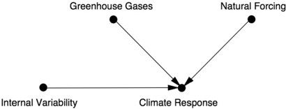
I am not personally an expert on climate change, so I got this example from one of my collaborators, Alexis Hannart of the Franco-Argentine Institute on the Study of Climate and Its Impacts in Buenos Aires, who has been a big proponent of causal analysis in climate science. Hannart draws the causal graph in Figure 8.4. Because Greenhouse Gases is a top-level node in the climate model, with no arrows going into it, he argues that there is no confounding between it and Climate Response. Likewise, he vouches for the no-protection assumption (i.e., greenhouse gases cannot protect us from heat waves).

Hannart goes beyond Allen and Stott and uses our formulas to compute the probability of sufficiency ( PS ) and of necessity ( PN ). In the case of the 2003 European heat wave, he finds that PS was extremely low, about 0.0072, meaning that there was no way to predict that this event would happen in this particular year. On the other hand, the probability of necessity PN was 0.9, in agreement with Allen and Stott's results. This means that it is highly likely that, without greenhouse gases, the heat wave would not have happened.

The apparently low value of PS has to be put into a larger context. We don't just want to know the probability of a heat wave this year; we would like to know the probability of a recurrence of such a severe heat wave over a longer time frame-say in the next ten or fifty years. As the time frame lengthens, PN decreases because other possible mechanisms for a heat wave might come into play. On the other hand, PS increases because we are in effect giving the dice more chances to come up snake eyes. So, for example, Hannart computes that there is an 80 percent probability that climate change will be a sufficient cause of another European heat wave like the 2003 one (or worse) in a two-hundred-year period. That might not sound too terrifying, but that's assuming the greenhouse gas levels of today. In reality, CO levels are 2 certain to continue rising, which can only increase PS and shorten the window of time until the next heat wave.

FIGURE 8.4. Causal diagram for the climate change example.

Can ordinary people learn to understand the difference between necessary and sufficient causes? This is a nontrivial question. Even scientists sometimes struggle. In fact, two conflicting studies came out that analyzed the 2010 heat wave in Russia, when Russia had its hottest summer ever and peat fires darkened the skies of Moscow. One group concluded that natural variability caused the heat wave; another concluded that climate change caused it. In all likelihood, the disagreement occurred because the two groups defined their outcome differently. One group apparently based its argument on PN and got a high likelihood that climate change was the cause, while the other used PS and got a low likelihood. The second group attributed the heat wave to a persistent high-pressure or 'blocking pattern' over Russia-which sounds to me like a sufficient cause-and found that greenhouse gases had little to do

with this phenomenon. But any study that uses PS as a metric, over a short period, is setting a high bar for proving causation.

Before leaving this example, I would like to comment again on the computer models. Most other scientists have to work very hard to get counterfactual information, for example by painfully combining data from observational and experimental studies. Climate scientists can get counterfactuals very easily from their computer models: just enter in a new number for the carbon dioxide concentration and let the program run. 'Easily' is, of course, relative. Behind the simple causal diagram of Figure 8.4 lies a fabulously complex response function, given by the millions of lines of computer code that go into a climate simulation.

This brings up a natural question: How much can we trust the computer simulations? The question has political ramifications, especially here in the United States. However, I will try to give an apolitical answer. I would consider the response function in this example much more credible than the linear models that one sees so often in natural and social sciences. Linear models are often chosen for no good reason other than convenience. By comparison, the climate models reflect more than a century of study by physicists, meteorologists, and climate scientists. They represent the best efforts of a community of scientists to understand the processes that govern our weather and climate. By any normal scientific standards, the climate models are strong and compelling evidence, but with one caveat. Though they are excellent at forecasting the weather a few days ahead, they have never been verified in a prospective trial over century-long timescales, so they could still contain systematic errors that we don't know about.

A WORLD OF COUNTERFACTUALS

I hope that by now it is obvious that counterfactuals are an essential part of how humans learn about the world and how our actions affect it. While we can never walk down both the paths that diverge in a wood, in a great many cases we can know, with some degree of confidence, what lies down each.

Beyond doubt, the variety and richness of causal queries that we can pose to our 'inference engine' are greatly enhanced when we can include counterfactuals in the mix. Another very popular kind of query, which I have not discussed here, called the effect of treatment on the treated (ETT), is used to evaluate whether people who gain access to a treatment are those who would benefit most from it. This measure is in many cases superior to the

conventional measure of a treatment's effectiveness, the average causal effect (ACE). The ACE, which you can get from a randomized controlled trial, averages treatment efficacy over the entire population. But what if, in actual implementation, those recruited for a treatment program are the ones least likely to benefit from it? To assess the overall effectiveness of the program, ETT measures how adversely treated patients would be affected had they not been treated-a counterfactual measure of critical significance in practical decision making. My former student Ilya Shpitser (now at Johns Hopkins) has now done for ETT what the do -calculus did for ACE-provided a complete understanding of when it is estimable from data, given a causal diagram.

Undoubtedly the most popular application of counterfactuals in science today is called mediation analysis. For that reason, I devote a separate chapter to it (Chapter 9). Oddly, many people, especially if using classical mediation analysis techniques, may not realize that they are talking about a counterfactual effect.

In a scientific context, a mediator, or mediating variable, is one that transmits the effect of the treatment to the outcome. We have seen many mediation examples in this book, such as Smoking Tar Cancer (where Tar is the mediator). The main question of interest in such cases is whether the mediating variable accounts for the entire effect of the treatment variable or some part of the effect does not require a mediator. We would represent such an effect by a separate arrow leading directly from the treatment to the outcome, such as Smoking Cancer.

Mediation analysis aims to disentangle the direct effect (which does not pass through the mediator) from the indirect effect (the part that passes through the mediator). The importance is easy to see. If smoking causes lung cancer only through the formation of tar deposits, then we could eliminate the excess cancer risk by giving smokers tar-free cigarettes, such as e-cigarettes. On the other hand, if smoking causes cancer directly or through a different mediator, then e-cigarettes might not solve the problem. At present this medical question is unresolved.

At this point it is probably not obvious to you that direct and indirect effects involve counterfactual statements. It was definitely not obvious to me! In fact, it was one of the biggest surprises of my career. The next chapter tells this story and gives many real-life applications of mediation analysis.

In 1912, a cairn of snow and a cross of skis mark the final resting place of Captain Robert Falcon Scott (right) and the last two men from his ill-fated expedition to the South Pole. Among numerous hardships, Scott's men suffered from scurvy. This part of the tragedy could have been averted if scientists had understood the mechanism by which citrus fruits prevent the disease. ( Source: left, photograph by Tryggve Gran (presumed); right, photograph by Herbert Ponting. Courtesy of

Canterbury Museum, New Zealand.)