Chapter 4: Confounding and Deconfounding: Or, Slaying the Lurking Variable
If our conception of causal effects had anything to do with randomized experiments, the latter would have been invented 500 years before Fisher.
-THE AUTHOR (2016)
ASHPENAZ, the overseer of King Nebuchadnezzar's court, had a major problem. In 597 BC, the king of Babylon had sacked the kingdom of Judah and brought back thousands of captives, many of them the nobility of Jerusalem. As was customary in his kingdom, Nebuchadnezzar wanted some of them to serve in his court, so he commanded Ashpenaz to seek out 'children in whom was no blemish, but well favoured, and skilful in all wisdom, and cunning in knowledge, and understanding science.' These lucky children were to be educated in the language and culture of Babylon so that they could serve in the administration of the empire, which stretched from the Persian Gulf to the Mediterranean Sea. As part of their education, they would get to eat royal meat and drink royal wine.
And therein lay the problem. One of his favorites, a boy named Daniel, refused to touch the food. For religious reasons, he could not eat meat not prepared according to Jewish laws, and he asked that he and his friends be given a diet of vegetables instead. Ashpenaz would have liked to comply with
the boy's wishes, but he was afraid that the king would notice: 'Once he sees your frowning faces, different from the other children your age, it will cost me my head.'
Daniel tried to assure Ashpenaz that the vegetarian diet would not diminish their capacity to serve the king. As befits a person 'cunning in knowledge, and understanding science,' he proposed an experiment. Try us for ten days, he said. Take four of us and feed us only vegetables; take another group of children and feed them the king's meat and wine. After ten days, compare the two groups. Said Daniel, 'And as thou seest, deal with thy servants.'
Even if you haven't read the story, you can probably guess what happened next. Daniel and his three companions prospered on the vegetarian diet. The king was so impressed with their wisdom and learning-not to mention their healthy appearance-that he gave them a favored place in his court, where 'he found them ten times better than all the magicians and astrologers that were in all his realm.' Later Daniel became an interpreter of the king's dreams and survived a memorable encounter in a lion's den.
Believe it or not, the biblical story of Daniel encapsulates in a profound way the conduct of experimental science today. Ashpenaz asks a question about causation: Will a vegetarian diet cause my servants to lose weight? Daniel proposes a methodology to deal with any such questions: Set up two groups of people, identical in all relevant ways. Give one group a new treatment (a diet, a drug, etc.), while the other group (called the control group) either gets the old treatment or no special treatment at all. If, after a suitable amount of time, you see a measurable difference between the two supposedly identical groups of people, then the new treatment must be the cause of the difference.
Nowadays we call this a controlled experiment. The principle is simple. To understand the causal effect of the diet, we would like to compare what happens to Daniel on one diet with what would have happened if he had stayed on the other. But we can't go back in time and rewrite history, so instead we do the next best thing: we compare a group of people who get the treatment with a group of similar people who don't. It's obvious, but nevertheless crucial, that the groups be comparable and representative of some population. If these conditions are met, then the results should be transferable to the population at large. To Daniel's credit, he seems to understand this. He isn't just asking for vegetables on his own behalf: if the trial shows the vegetarian diet is better, then all the Israelite servants should
be allowed that diet in the future. That, at least, is how I interpret the phrase, 'As thou seest, deal with thy servants.'
Daniel also understood that it was important to compare groups. In this respect he was already more sophisticated than many people today, who choose a fad diet (for example) just because a friend went on that diet and lost weight. If you choose a diet based only on one friend's experience, you are essentially saying that you believe you are similar to your friend in all relevant details: age, heredity, home environment, previous diet, and so forth. That is a lot to assume.
Another key point of Daniel's experiment is that it was prospective: the groups were chosen in advance. By contrast, suppose that you see twenty people in an infomercial who all say they lost weight on a diet. That seems like a pretty large sample size, so some viewers might consider it convincing evidence. But that would amount to basing their decision on the experience of people who already had a good response. For all you know, for every person who lost weight, ten others just like him or her tried the diet and had no success. But of course, they weren't chosen to appear on the infomercial.
Daniel's experiment was strikingly modern in all these ways. Prospective controlled trials are still a hallmark of sound science. However, Daniel didn't think of one thing: confounding bias. Suppose that Daniel and his friends are healthier than the control group to start with. In that case, their robust appearance after ten days on the diet may have nothing to do with the diet itself; it may reflect their overall health. Maybe they would have prospered even more if they had eaten the king's meat!
Confounding bias occurs when a variable influences both who is selected for the treatment and the outcome of the experiment. Sometimes the confounders are known; other times they are merely suspected and act as a 'lurking third variable.' In a causal diagram, confounders are extremely easy to recognize: in Figure 4.1, the variable Z at the center of the fork is a confounder of X and Y . (We will see a more universal definition later, but this triangle is the most recognizable and common situation.)
FIGURE 4.1. The most basic version of confounding: Z is a confounder of the proposed causal relationship between X and Y .
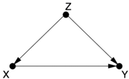
The term 'confounding' originally meant 'mixing' in English, and we can understand from the diagram why this name was chosen. The true causal effect X Y is 'mixed' with the spurious correlation between X and Y induced by the fork X Z Y . For example, if we are testing a drug and give it to patients who are younger on average than the people in the control group, then age becomes a confounder-a lurking third variable. If we don't have any data on the ages, we will not be able to disentangle the true effect from the spurious effect.
However, the converse is also true. If we do have measurements of the third variable, then it is very easy to deconfound the true and spurious effects. For instance, if the confounding variable Z is age, we compare the treatment and control groups in every age group separately. We can then take an average of the effects, weighting each age group according to its percentage in the target population. This method of compensation is familiar to all statisticians; it is called 'adjusting for Z ' or 'controlling for Z .'
Oddly, statisticians both over- and underrate the importance of adjusting for possible confounders. They overrate it in the sense that they often control for many more variables than they need to and even for variables that they should not control for. I recently came across a quote from a political blogger named Ezra Klein who expresses this phenomenon of 'overcontrolling' very clearly: 'You see it all the time in studies. 'We controlled for…' And then the list starts. The longer the better. Income. Age. Race. Religion. Height. Hair color. Sexual preference. Crossfit attendance. Love of parents. Coke or Pepsi. The more things you can control for, the stronger your study is-or, at least, the stronger your study seems. Controls give the feeling of specificity, of precision.… But sometimes, you can control for too much. Sometimes you end up controlling for the thing you're trying to measure.' Klein raises a valid concern. Statisticians have been immensely confused about what variables should and should not be controlled for, so the default practice has been to control for everything one can measure. The vast majority of studies conducted in this day and age subscribe to this practice. It is a convenient, simple procedure to follow, but it is both wasteful and ridden with errors. A key achievement of the Causal Revolution has been to bring an end to this confusion.
At the same time, statisticians greatly underrate controlling in the sense that they are loath to talk about causality at all, even if the controlling has been done correctly. This too stands contrary to the message of this chapter: if you have identified a sufficient set of deconfounders in your diagram, gathered data on them, and properly adjusted for them, then you have every
right to say that you have computed the causal effect X Y (provided, of course, that you can defend your causal diagram on scientific grounds).
The textbook approach of statisticians to confounding is quite different and rests on an idea most effectively advocated by R. A. Fisher: the randomized controlled trial (RCT). Fisher was exactly right, but not for exactly the right reasons. The randomized controlled trial is indeed a wonderful invention-but until recently the generations of statisticians who followed Fisher could not prove that what they got from the RCT was indeed what they sought to obtain. They did not have a language to write down what they were looking for-namely, the causal effect of X on Y . One of my goals in this chapter is to explain, from the point of view of causal diagrams, precisely why RCTs allow us to estimate the causal effect X Y without falling prey to confounder bias. Once we have understood why RCTs work, there is no need to put them on a pedestal and treat them as the gold standard of causal analysis, which all other methods should emulate. Quite the opposite: we will see that the so-called gold standard in fact derives its legitimacy from more basic principles.
This chapter will also show that causal diagrams make possible a shift of emphasis from confounders to deconfounders. The former cause the problem; the latter cure it. The two sets may overlap, but they don't have to. If we have data on a sufficient set of deconfounders, it does not matter if we ignore some or even all of the confounders.
This shift of emphasis is a main way in which the Causal Revolution allows us to go beyond Fisherian experiments and infer causal effects from nonexperimental studies. It enables us to determine which variables should be controlled for to serve as deconfounders. This question has bedeviled both theoretical and practical statisticians; it has been an Achilles' heel of the field for decades. That is because it has nothing to do with data or statistics. Confounding is a causal concept-it belongs on rung two of the Ladder of Causation.
Graphical methods, beginning in the 1990s, have totally deconfounded the confounding problem. In particular, we will soon meet a method called the back-door criterion, which unambiguously identifies which variables in a causal diagram are deconfounders. If the researcher can gather data on those variables, she can adjust for them and thereby make predictions about the result of an intervention even without performing it.
In fact, the Causal Revolution has gone even farther than this. In some cases we can control for confounding even when we do not have data on a
sufficient set of deconfounders. In these cases we can use different adjustment formulas-not the conventional one, which is only appropriate for use with the back-door criterion-and still eradicate all confounding. We will save these exciting developments for Chapter 7.
Although confounding has a long history in all areas of science, the recognition that the problem requires causal, not statistical, solutions is very recent. Even as recently as 2001, reviewers rebuked a paper of mine while insisting, 'Confounding is solidly founded in standard statistics.' Fortunately, the number of such reviewers has shrunk dramatically in the past decade. There is now an almost universal consensus, at least among epidemiologists, philosophers, and social scientists, that (1) confounding needs and has a causal solution, and (2) causal diagrams provide a complete and systematic way of finding that solution. The age of confusion over confounding has come to an end!
THE CHILLING FEAR OF CONFOUNDING
In 1998, a study in the New England Journal of Medicine revealed an association between regular walking and reduced death rates among retired men. The researchers used data from the Honolulu Heart Program, which has followed the health of 8,000 men of Japanese ancestry since 1965.
The researchers, led by Robert Abbott, a biostatistician at the University of Virginia, wanted to know whether the men who exercised more lived longer. They chose a sample of 707 men from the larger group of 8,000, all of whom were physically healthy enough to walk. Abbott's team found that the death rate over a twelve-year period was two times higher among men who walked less than a mile a day (I'll call them 'casual walkers') than among men who walked more than two miles a day ('intense walkers'). To be precise, 43 percent of the casual walkers had died, while only 21.5 percent of the intense walkers had died.
However, because the experimenters did not prescribe who would be a casual walker and who would be an intense walker, we have to take into consideration the possibility of confounding bias. An obvious confounder might be age: younger men might be more willing to do a vigorous workout and also would be less likely to die. So we would have a causal diagram like that in Figure 4.2.
FIGURE 4.2. Causal diagram for walking example.
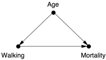
The classic forking pattern at the 'Age' node tells us that age is a confounder of walking and mortality. I'm sure you can think of other possible confounders. Perhaps the casual walkers were slacking off for a reason; maybe they couldn't walk as much. Thus, physical condition could be a confounder. We could go on and on like this. What if the light walkers were alcohol drinkers? What if they ate more?
The good news is, the researchers thought about all these factors. The study has accounted and adjusted for every reasonable factor-age, physical condition, alcohol consumption, diet, and several others. For example, it's true that the intense walkers tended to be slightly younger. So the researchers adjusted the death rate for age and found that the difference between casual and intense walkers was still very large. (The age-adjusted death rate for the casual walkers was 41 percent, compared to 24 percent for the intense walkers.)
Even so, the researchers were very circumspect in their conclusions. At the end of the article, they wrote, 'Of course, the effects on longevity of intentional efforts to increase the distance walked per day by physically capable older men cannot be addressed in our study.' To use the language of Chapter 1, they decline to say anything about your probability of surviving twelve years given that you do exercise ( ).
In fairness to Abbott and the rest of his team, they may have had good reasons for caution. This was a first study, and the sample was relatively small and homogeneous. Nevertheless, this caution reflects a more general attitude, transcending issues of homogeneity and sample size. Researchers have been taught to believe that an observational study (one where subjects choose their own treatment) can never illuminate a causal claim. I assert that this caution is overexaggerated. Why else would one bother adjusting for all these confounders, if not to get rid of the spurious part of the association and thereby get a better view of the causal part?
Instead of saying 'Of course we can't,' as they did, we should proclaim that of course we can say something about an intentional intervention. If we believe that Abbott's team identified all the important confounders, we must also believe that intentional walking tends to prolong life (at least in Japanese
males).
This provisional conclusion, predicated on the assumption that no other confounders could play a major role in the relationships found, is an extremely valuable piece of information. It tells a potential walker precisely what kind of uncertainty remains in taking the claim at face value. It tells him that the remaining uncertainty is not higher than the possibility that additional confounders exist that were not taken into account. It is also valuable as a guide to future studies, which should focus on those other factors (if they exist), not the ones neutralized in the current study. In short, knowing the set of assumptions that stand behind a given conclusion is not less valuable than attempting to circumvent those assumptions with an RCT, which, as we shall see, has complications of its own.
THE SKILLFUL INTERROGATION OF NATURE: WHY RCTS WORK
As I have mentioned already, the one circumstance under which scientists will abandon some of their reticence to talk about causality is when they have conducted a randomized controlled trial. You can read it on Wikipedia or in a thousand other places: 'The RCT is often considered the gold standard of a clinical trial.' We have one person to thank for this, R. A. Fisher, so it is very interesting to read what a person very close to him wrote about his reasons. The passage is lengthy, but worth quoting in full:
The whole art and practice of scientific experimentation is comprised in the skillful interrogation of Nature. Observation has provided the scientist with a picture of Nature in some aspect, which has all the imperfections of a voluntary statement. He wishes to check his interpretation of this statement by asking specific questions aimed at establishing causal relationships. His questions, in the form of experimental operations, are necessarily particular, and he must rely on the consistency of Nature in making general deductions from her response in a particular instance or in predicting the outcome to be anticipated from similar operations on other occasions. His aim is to draw valid conclusions of determinate precision and generality from the evidence he elicits.
Far from behaving consistently, however, Nature appears vacillating, coy, and ambiguous in her answers. She responds to the form of the question as it is set out in the field and not necessarily to
the question in the experimenter's mind; she does not interpret for him; she gives no gratuitous information; and she is a stickler for accuracy. In consequence, the experimenter who wants to compare two manurial treatments wastes his labor if, dividing his field into two equal parts, he dresses each half with one of his manures, grows a crop, and compares the yields from the two halves. The form of his question was: what is the difference between the yield of plot A under the first treatment and that of plot B under the second? He has not asked whether plot A would yield the same as plot B under uniform treatment, and he cannot distinguish plot effects from treatment effects, for Nature has recorded, as requested, not only the contribution of the manurial differences to the plot yields but also the contributions of differences in soil fertility, texture, drainage, aspect, microflora, and innumerable other variables.
The author of this passage is Joan Fisher Box, the daughter of Ronald Aylmer Fisher, and it is taken from her biography of her illustrious father. Though not a statistician herself, she has clearly absorbed very deeply the central challenge statisticians face. She states in no uncertain terms that the questions they ask are 'aimed at establishing causal relationships.' And what gets in their way is confounding, although she does not use that word. They want to know the effect of a fertilizer (or 'manurial treatment,' as fertilizers were called in that era)-that is, the expected yield under one fertilizer compared with the yield under an alternative. Nature, however, tells them about the effect of the fertilizer mixed (remember, this is the original meaning of 'confounded') with a variety of other causes.
I like the image that Fisher Box provides in the above passage: Nature is like a genie that answers exactly the question we pose, not necessarily the one we intend to ask. But we have to believe, as Fisher Box clearly does, that the answer to the question we wish to ask does exist in nature. Our experiments are a sloppy means of uncovering the answer, but they do not by any means define the answer. If we follow her analogy exactly, then do X ( = x ) must come first, because it is a property of nature that represents the answer we seek: What is the effect of using the first fertilizer on the whole field? Randomization comes second, because it is only a man-made means to elicit the answer to that question. One might compare it to the gauge on a thermometer, which is a means to elicit the temperature but is not the temperature itself.
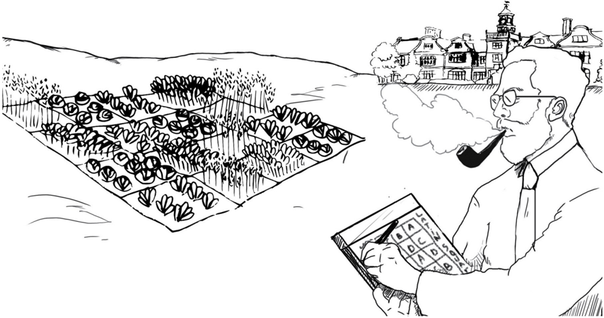
In his early years at Rothamsted Experimental Station, Fisher usually took a very elaborate, systematic approach to disentangling the effects of fertilizer from other variables. He would divide his fields into a grid of subplots and
plan carefully so that each fertilizer was tried with each combination of soil type and plant (see Figure 4.3). He did this to ensure the comparability of each sample; in reality, he could never anticipate all the confounders that might determine the fertility of a given plot. A clever enough genie could defeat any structured layout of the field.
Around 1923 or 1924, Fisher began to realize that the only experimental design that the genie could not defeat was a random one. Imagine performing the same experiment one hundred times on a field with an unknown distribution of fertility. Each time you assign fertilizers to subplots randomly. Sometimes you may be very unlucky and use Fertilizer 1 in all the least fertile subplots. Other times you may get lucky and apply it to the most fertile subplots. But by generating a new random assignment each time you perform the experiment, you can guarantee that the great majority of the time you will be neither lucky nor unlucky. In those cases, Fertilizer 1 will be applied to a selection of subplots that is representative of the field as a whole. This is exactly what you want for a controlled trial. Because the distribution of fertility in the field is fixed throughout your series of experiments-the genie can't change it-he is tricked into answering (most of the time) the causal question you wanted to ask.
FIGURE 4.3. R. A. Fisher with one of his many innovations: a Latin square experimental design, intended to ensure that one plot of each plant type appears in each row (fertilizer type) and column (soil type). Such designs are still used in practice, but Fisher would later argue convincingly that a randomized design is even more effective. ( Source: Drawing by Dakota Harr.)
From our perspective, in an era when randomized trials are the gold standard, all of this may appear obvious. But at the time, the idea of a randomly designed experiment horrified Fisher's statistical colleagues. Fisher's literally drawing from a deck of cards to assign subplots to each fertilizer may have contributed to their dismay. Science subjected to the whims of chance?
But Fisher realized that an uncertain answer to the right question is much better than a highly certain answer to the wrong question. If you ask the genie the wrong question, you will never find out what you want to know. If you ask the right question, getting an answer that is occasionally wrong is much less of a problem. You can still estimate the amount of uncertainty in your answer, because the uncertainty comes from the randomization procedure (which is known) rather than the characteristics of the soil (which are unknown).
Thus, randomization actually brings two benefits. First, it eliminates confounder bias (it asks Nature the right question). Second, it enables the researcher to quantify his uncertainty. However, according to historian Stephen Stigler, the second benefit was really Fisher's main reason for advocating randomization. He was the world's master of quantifying uncertainty, having developed many new mathematical procedures for doing so. By comparison, his understanding of deconfounding was purely intuitive, for he lacked a mathematical notation for articulating what he sought.
Now, ninety years later, we can use the do -operator to fill in what Fisher wanted to but couldn't ask. Let's see, from a causal point of view, how randomization enables us to ask the genie the right question.
Let's start, as usual, by drawing a causal diagram. Model 1, shown in Figure 4.4, describes how the yield of each plot is determined under normal conditions, where the farmer decides by whim or bias which fertilizer is best for each plot. The query he wants to pose to the genie Nature is 'What is the yield under a uniform application of Fertilizer 1 (versus Fertilizer 2) to the entire field?' Or, in do -operator notation, what is P yield ( | do fertilizer ( = 1))?
FIGURE 4.4. Model 1: an improperly controlled experiment.
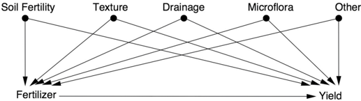
If the farmer performs the experiment naively, for example applying
Fertilizer 1 to the high end of his field and Fertilizer 2 to the low end, he is probably introducing Drainage as a confounder. If he uses Fertilizer 1 one year and Fertilizer 2 the next year, he is probably introducing Weather as a confounder. In either case, he will get a biased comparison.
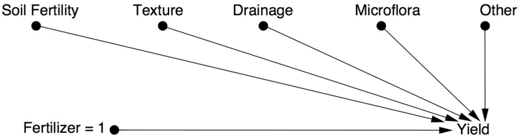
The world that the farmer wants to know about is described by Model 2, where all plots receive the same fertilizer (see Figure 4.5). As explained in Chapter 1, the effect of the do -operator is to erase all the arrows pointing to Fertilizer and force this variable to a particular value-say, Fertilizer = 1.
FIGURE 4.5. Model 2: the world we would like to know about.
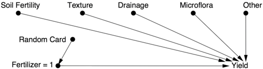
Finally, let's see what the world looks like when we apply randomization. Now some plots will be subjected to do fertilizer ( = 1) and others to do fertilizer ( = 2), but the choice of which treatment goes to which plot is random. The world created by such a model is shown by Model 3 in Figure 4.6, showing the variable Fertilizer obtaining its assignment by a random device-say, Fisher's deck of cards.
Notice that all the arrows pointing toward Fertilizer have been erased, reflecting the assumption that the farmer listens only to the card when deciding which fertilizer to use. It is equally important to note that there is no arrow from Card to Yield, because the plants cannot read the cards. (This is a fairly safe assumption for plants, but for human subjects in a randomized trial it is a serious concern.) Therefore Model 3 describes a world in which the relation between Fertilizer and Yield is unconfounded (i.e., there is no common cause of Fertilizer and Yield). This means that in the world described by Figure 4.6, there is no difference between seeing Fertilizer = 1 and doing Fertilizer = 1.
FIGURE 4.6. Model 3: the world simulated by a randomized controlled trial.
That brings us to the punch line: randomization is a way of simulating Model 2. It disables all the old confounders without introducing any new
confounders. That is the source of its power; there is nothing mysterious or mystical about it. It is nothing more or less than, as Joan Fisher Box said, 'the skillful interrogation of Nature.'
The experiment would, however, fail in its objective of simulating Model 2 if either the experimenter were allowed to use his own judgment to choose a fertilizer or the experimental subjects, in this case the plants, 'knew' which card they had drawn. This is why clinical trials with human subjects go to great lengths to conceal this information from both the patients and the experimenters (a procedure known as double blinding).
I will add to this a second punch line: there are other ways of simulating Model 2. One way, if you know what all the possible confounders are, is to measure and adjust for them. However, randomization does have one great advantage: it severs every incoming link to the randomized variable, including the ones we don't know about or cannot measure (e.g., 'Other' factors in Figures 4.4 to 4.6).
By contrast, in a nonrandomized study, the experimenter must rely on her knowledge of the subject matter. If she is confident that her causal model accounts for a sufficient number of deconfounders and she has gathered data on them, then she can estimate the effect of Fertilizer on Yield in an unbiased way. But the danger is that she may have missed a confounding factor, and her estimate may therefore be biased.
All things being equal, RCTs are still preferred to observational studies, just as safety nets are recommended for tightrope walkers. But all things are not necessarily equal. In some cases, intervention may be physically impossible (for instance, in a study of the effect of obesity on heart disease, we cannot randomly assign patients to be obese or not). Or intervention may be unethical (in a study of the effects of smoking, we can't ask randomly selected people to smoke for ten years). Or we may encounter difficulties recruiting subjects for inconvenient experimental procedures and end up with volunteers who do not represent the intended population.
Fortunately, the do -operator gives us scientifically sound ways of determining causal effects from nonexperimental studies, which challenge the traditional supremacy of RCTs. As discussed in the walking example, such causal estimates produced by observational studies may be labeled 'provisional causality,' that is, causality contingent upon the set of assumptions that our causal diagram advertises. It is important that we not treat these studies as second-class citizens: they have the advantage of being conducted in the natural habitat of the target population, not in the artificial
setting of a laboratory, and they can be 'pure' in the sense of not being contaminated by issues of ethics or feasibility.
Now that we understand that the principal objective of an RCT is to eliminate confounding, let's look at the other methods that the Causal Revolution has given us. The story begins with a 1986 paper by two of my longtime colleagues, which started a reevaluation of what confounding means.
THE NEW PARADIGM OF CONFOUNDING
'While confounding is widely recognized as one of the central problems in epidemiological research, a review of the literature will reveal little consistency among the definitions of confounding or confounder.' With this one sentence, Sander Greenland of the University of California, Los Angeles, and Jamie Robins of Harvard University put their finger on the central reason why the control of confounding had not advanced one bit since Fisher. Lacking a principled understanding of confounding, scientists could not say anything meaningful in observational studies where physical control over treatments is infeasible.
How was confounding defined then, and how should it be defined? Armed with what we now know about the logic of causality, the answer to the second question is easier. The quantity we observe is the conditional probability of the outcome given the treatment, P Y ( | X ). The question we want to ask of Nature has to do with the causal relationship between X and Y , which is captured by the interventional probability P Y ( | do X ( )). Confounding, then, should simply be defined as anything that leads to a discrepancy between the two: P Y ( | X ) ≠ P Y ( | do X ( )). Why all the fuss?
Unfortunately, things were not as easy as that before the 1990s because the do -operator had yet to be formalized. Even today, if you stop a statistician in the street and ask, 'What does 'confounding' mean to you?' you will probably get one of the most convoluted and confounded answers you ever heard from a scientist. One recent book, coauthored by leading statisticians, spends literally two pages trying to explain it, and I have yet to find a reader who understood the explanation.
The reason for the difficulty is that confounding is not a statistical notion. It stands for the discrepancy between what we want to assess (the causal effect) and what we actually do assess using statistical methods. If you can't
articulate mathematically what you want to assess, you can't expect to define what constitutes a discrepancy.
Historically, the concept of 'confounding' has evolved around two related conceptions: incomparability and a lurking third variable. Both of these concepts have resisted formalization. When we talked about comparability, in the context of Daniel's experiment, we said that the treatment and control groups should be identical in all relevant ways. But this begs us to distinguish relevant from irrelevant attributes. How do we know that age is relevant in the Honolulu walking study? How do we know that the alphabetical order of a participant's name is not relevant? You might say it's obvious or common sense, but generations of scientists have struggled to articulate that common sense formally, and a robot cannot rely on our common sense when asked to act properly.
The same ambiguity plagues the third-variable definition. Should a confounder be a common cause of both X and Y or merely correlated with each? Today we can answer such questions by referring to the causal diagram and checking which variables produce a discrepancy between P X ( | Y ) and P X ( | do Y ( )). Lacking a diagram or a do -operator, five generations of statisticians and health scientists had to struggle with surrogates, none of which were satisfactory. Considering that the drugs in your medicine cabinet may have been developed on the basis of a dubious definition of 'confounders,' you should be somewhat concerned.
Let's take a look at some of the surrogate definitions of confounding. These fall into two main categories, declarative and procedural. A typical (and wrong) declarative definition would be 'A confounder is any variable that is correlated with both X and Y .' On the other hand, a procedural definition would attempt to characterize a confounder in terms of a statistical test. This appeals to statisticians, who love any test that can be performed on the data directly without appealing to a model.
Here is a procedural definition that goes by the scary name of 'noncollapsibility.' It comes from a 1996 paper by the Norwegian epidemiologist Sven Hernberg: 'Formally one can compare the crude relative risk and the relative risk resulting after adjustment for the potential confounder. A difference indicates confounding, and in that case one should use the adjusted risk estimate. If there is no or a negligible difference, confounding is not an issue and the crude estimate is to be preferred.' In other words, if you suspect a confounder, try adjusting for it and try not adjusting for it. If there is a difference, it is a confounder, and you should trust the
adjusted value. If there is no difference, you are off the hook. Hernberg was by no means the first person to advocate such an approach; it has misguided a century of epidemiologists, economists, and social scientists, and it still reigns in certain quarters of applied statistics. I have picked on Hernberg only because he was unusually explicit about it and because he wrote this in 1996, well after the Causal Revolution was already underway.
The most popular of the declarative definitions evolved over a period of time. Alfredo Morabia, author of A History of Epidemiologic Methods and Concepts , calls it 'the classic epidemiological definition of confounding,' and it consists of three parts. A confounder of X (the treatment) and Y (the outcome) is a variable Z that is (1) associated with X in the population at large, and (2) associated with Y among people who have not been exposed to the treatment X . In recent years, this has been supplemented by a third condition: (3) Z should not be on the causal path between X and Y .
Observe that all the terms in the 'classic' version (1 and 2) are statistical. In particular, Z is only assumed to be associated with-not a cause ofX and Y . Edward Simpson proposed the rather convoluted condition ' Y is associated with Z among the unexposed' in 1951. From the causal point of view, it seems that Simpson's idea was to discount the part of the correlation of Z with Y that is due to the causal effect of X on Y ; in other words, he wanted to say that Z has an effect on Y independent of its effect on X . The only way he could think to express this discounting was to condition on X by focusing on the control group ( X = 0). Statistical vocabulary, deprived of the word 'effect,' gave him no other way of saying it.
If this is a bit confusing, it should be! How much easier it would have been if he could have simply written a causal diagram, like Figure 4.1, and said, ' Y is associated with Z via paths not going through X .' But he didn't have this tool, and he couldn't talk about paths, which were a forbidden concept.
The 'classical epidemiological definition' of a confounder has other flaws, as the following two examples show:
and
In example (i), Z satisfies conditions (1) and (2) but is not a confounder. It is known as a mediator: it is the variable that explains the causal effect of X
on Y . It is a disaster to control for Z if you are trying to find the causal effect of X on Y . If you look only at those individuals in the treatment and control groups for whom Z = 0, then you have completely blocked the effect of X , because it works by changing Z . So you will conclude that X has no effect on Y . This is exactly what Ezra Klein meant when he said, 'Sometimes you end up controlling for the thing you're trying to measure.'
In example (ii), Z is a proxy for the mediator M . Statisticians very often control for proxies when the actual causal variable can't be measured; for instance, party affiliation might be used as a proxy for political beliefs. Because Z isn't a perfect measure of M , some of the influence of X on Y might 'leak through' if you control for Z . Nevertheless, controlling for Z is still a mistake. While the bias might be less than if you controlled for M , it is still there.
For this reason later statisticians, notably David Cox in his textbook The Design of Experiments (1958), warned that you should only control for Z if you have a 'strong prior reason' to believe that it is not affected by X . This 'strong prior reason' is nothing more or less than a causal assumption. He adds, 'Such hypotheses may be perfectly in order, but the scientist should always be aware when they are being appealed to.' Remember that it's 1958, in the midst of the great prohibition on causality. Cox is saying that you can go ahead and take a swig of causal moonshine when adjusting for confounders, but don't tell the preacher. A daring suggestion! I never fail to commend him for his bravery.
By 1980, Simpson's and Cox's conditions had been combined into the three-part test for confounding that I mentioned above. It is about as trustworthy as a canoe with only three leaks. Even though it does make a halfhearted appeal to causality in part (3), each of the first two parts can be shown to be both unnecessary and insufficient.
Greenland and Robins drew that conclusion in their landmark 1986 paper. The two took a completely new approach to confounding, which they called 'exchangeability.' They went back to the original idea that the control group ( X = 0) should be comparable to the treatment group ( X = 1). But they added a counterfactual twist. (Remember from Chapter 1 that counterfactuals are at rung three of the Ladder of Causation and therefore powerful enough to detect confounding.) Exchangeability requires the researcher to consider the treatment group, imagine what would have happened to its constituents if they had not gotten treatment, and then judge whether the outcome would be the same as for those who (in reality) did not receive treatment. Only then can we
say that no confounding exists in the study.
In 1986, talking counterfactuals to an audience of epidemiologists took some courage, because they were still very much under the influence of classical statistics, which holds that all the answers are in the data-not in what might have been, which will remain forever unobserved. However, the statistical community was somewhat prepared to listen to such heresy, thanks to the pioneering work of another Harvard statistician, Donald Rubin. In Rubin's 'potential outcomes' framework, proposed in 1974, counterfactual variables like 'Blood Pressure of Person X had he received Drug D ' and 'Blood Pressure of Person X had he not received Drug D ' are just as legitimate as a traditional variable like Blood Pressure-despite the fact that one of those two variables will remain forever unobserved.
Robins and Greenland set out to express their conception of confounding in terms of potential outcomes. They partitioned the population into four types of individuals: doomed, causative, preventive, and immune. The language is suggestive, so let's think of the treatment X as a flu vaccination and the outcome Y as coming down with flu. The doomed people are those for whom the vaccine doesn't work; they will get flu whether they get the vaccine or not. The causative group (which may be nonexistent) includes those for whom the vaccine actually causes the disease. The preventive group consists of people for whom the vaccine prevents the disease: they will get flu if they are not vaccinated, and they will not get flu if they are vaccinated. Finally, the immune group consists of people who will not get flu in either case. Table 4.1 sums up these considerations.
Ideally, each person would have a sticker on his forehead identifying which group he belonged to. Exchangeability simply means that the percentage of people with each kind of sticker ( d percent, c percent, p percent, and i percent, respectively) should be the same in both the treatment and control groups. Equality among these proportions guarantees that the outcome would be just the same if we switched the treatments and controls. Otherwise, the treatment and control groups are not alike, and our estimate of the effect of the vaccine will be confounded. Note that the two groups may be different in many ways. They can differ in age, sex, health conditions, and a variety of other characteristics. Only equality among d , c , p , and i determines whether they are exchangeable or not. So exchangeability amounts to equality between two sets of four proportions, a vast reduction in complexity from the alternative of assessing the innumerable factors by which the two groups may differ.
TABLE 4.1. Classification of individuals according to response type.
Using this commonsense definition of confounding, Greenland and Robins showed that the 'statistical' definitions, both declarative and procedural, give incorrect answers. A variable can satisfy the three-part test of epidemiologists and still increase bias, if adjusted for.
Greenland and Robins's definition was a great achievement, because it enabled them to give explicit examples showing that the previous definitions of confounding were inadequate. However, the definition could not be translated into practice. To put it simply, those stickers on the forehead don't exist. We do not even have a count of the proportions d , c , p , and i . In fact, this is precisely the kind of information that the genie of Nature keeps locked inside her magic lantern and doesn't show to anybody. Lacking this information, the researcher is left to intuit whether the treatment and control groups are exchangeable or not.
By now, I hope that your curiosity is well piqued. How can causal diagrams turn this massive headache of confounding into a fun game? The trick lies in an operational test for confounding, called the back-door criterion. This criterion turns the problem of defining confounding, identifying confounders, and adjusting for them into a routine puzzle that is no more challenging than solving a maze. It has thus brought the thorny, age-old problem to a happy conclusion.
THE DO -OPERATOR AND THE BACK-DOOR CRITERION
To understand the back-door criterion, it helps first to have an intuitive sense of how information flows in a causal diagram. I like to think of the links as pipes that convey information from a starting point X to a finish Y . Keep in mind that the conveying of information goes in both directions, causal and noncausal, as we saw in Chapter 3.
In fact, the noncausal paths are precisely the source of confounding. Remember that I define confounding as anything that makes P Y ( | do X ( )) differ from P Y ( | X ). The do -operator erases all the arrows that come into X , and in this way it prevents any information about X from flowing in the noncausal direction. Randomization has the same effect. So does statistical adjustment, if we pick the right variables to adjust.
In the last chapter, we looked at three rules that tell us how to stop the flow of information through any individual junction. I will repeat them for emphasis:
- (a) In a chain junction, A B C , controlling for B prevents information about A from getting to C or vice versa.
- (b) Likewise, in a fork or confounding junction, A B C , controlling for B prevents information about A from getting to C or vice versa.
- (c) Finally, in a collider, A B C , exactly the opposite rules hold. The variables A and C start out independent, so that information about A tells you nothing about C . But if you control for B , then information starts flowing through the 'pipe,' due to the explainaway effect.
We must also keep in mind another fundamental rule:
- (d) Controlling for descendants (or proxies) of a variable is like 'partially' controlling for the variable itself. Controlling for a descendant of a mediator partly closes the pipe; controlling for a descendant of a collider partly opens the pipe.
Now, what if we have longer pipes with more junctions, like this:
$$A B C D E F G H I J ?$$ The answer is very simple: if a single junction is blocked, then J cannot 'find out' about A through this path. So we have many options to block communication between A and J : control for B , control for C , don't control for D (because it's a collider), control for E , and so forth. Any one of these is sufficient. This is why the usual statistical procedure of controlling for everything that we can measure is so misguided. In fact, this particular path is blocked if we don't control for anything! The colliders at D and G block the path without any outside help. Controlling for D and G would open this path and enable J to listen to A .
Finally, to deconfound two variables X and Y , we need only block every noncausal path between them without blocking or perturbing any causal
paths. More precisely, a back-door path is any path from X to Y that starts with an arrow pointing into X . X and Y will be deconfounded if we block every back-door path (because such paths allow spurious correlation between X and Y ). If we do this by controlling for some set of variables Z , we also need to make sure that no member of Z is a descendant of X on a causal path; otherwise we might partly or completely close off that path.
That's all there is to it! With these rules, deconfounding becomes so simple and fun that you can treat it like a game. I urge you to try a few examples just to get the hang of it and see how easy it is. If you still find it hard, be assured that algorithms exist that can crack all such problems in a matter of nanoseconds. In each case, the goal of the game is to specify a set of variables that will deconfound X and Y . In other words, they should not be descended from X , and they should block all the back-door paths.
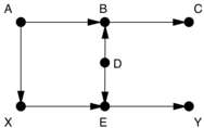
GAME 1.
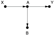
This one is easy! There are no arrows leading into X , therefore no backdoor paths. We don't need to control for anything.
Nevertheless, some researchers would consider B a confounder. It is associated with X because of the chain X A B . It is associated with Y among individuals with X = 0 because there is an open path B A Y that does not pass through X . And B is not on the causal path X A Y . It therefore passes the three-step 'classical epidemiological definition' for confounding, but it does not pass the back-door criterion and will lead to disaster if controlled for.
GAME 2.
In this example you should think of A , B , C , and D as 'pretreatment' variables. (The treatment, as usual, is X .) Now there is one back-door path X A B D E Y . This path is already blocked by the collider at B , so
we don't need to control for anything. Many statisticians would control for B or C , thinking there is no harm in doing so as long as they occur before the treatment. A leading statistician even recently wrote, 'To avoid conditioning on some observed covariates… is nonscientific ad hockery.' He is wrong; conditioning on B or C is a poor idea because it would open the noncausal path and therefore confound X and Y . Note that in this case we could reclose the path by controlling for A or D . This example shows that there may be different strategies for deconfounding. One researcher might take the easy way and not control for anything; a more traditional researcher might control for C and D . Both would be correct and should get the same result (provided that the model is correct, and we have a large enough sample).
GAME 3.
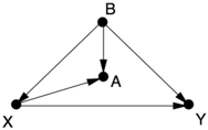
In Games 1 and 2 you didn't have to do anything, but this time you do. There is one back-door path from X to Y , X B Y , which can only be blocked by controlling for B . If B is unobservable, then there is no way of estimating the effect of X on Y without running a randomized controlled experiment. Some (in fact, most) statisticians in this situation would control for A , as a proxy for the unobservable variable B , but this only partially eliminates the confounding bias and introduces a new collider bias.
GAME 4.
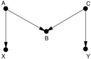
This one introduces a new kind of bias, called 'M-bias' (named for the shape of the graph). Once again there is only one back-door path, and it is already blocked by a collider at B . So we don't need to control for anything. Nevertheless, all statisticians before 1986 and many today would consider B a confounder. It is associated with X (via X A B ) and associated with Y via
a path that doesn't go through X B ( C Y ). It does not lie on a causal path and is not a descendant of anything on a causal path, because there is no causal path from X to Y . Therefore B passes the traditional three-step test for a confounder.
M-bias puts a finger on what is wrong with the traditional approach. It is incorrect to call a variable, like B , a confounder merely because it is associated with both X and Y . To reiterate, X and Y are unconfounded if we do not control for B B . only becomes a confounder when you control for it!
When I started showing this diagram to statisticians in the 1990s, some of them laughed it off and said that such a diagram was extremely unlikely to occur in practice. I disagree! For example, seat-belt usage ( B ) has no causal effect on smoking ( X ) or lung disease ( Y ); it is merely an indicator of a person's attitudes toward societal norms ( A ) as well as safety and healthrelated measures ( C ). Some of these attitudes may affect susceptibility to lung disease ( Y ). In practice, seatbelt usage was found to be correlated with both X and Y ; indeed, in a study conducted in 2006 as part of a tobacco litigation, seat-belt usage was listed as one of the first variables to be controlled for. If you accept the above model, then controlling for B alone would be a mistake.
Note that it's all right to control for B if you also control for A or C . Controlling for the collider B opens the 'pipe,' but controlling for A or C closes it again. Unfortunately, in the seat-belt example, A and C are variables relating to people's attitudes and not likely to be observable. If you can't observe it, you can't adjust for it.
GAME 5.
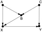
Game 5 is just Game 4 with a little extra wrinkle. Now a second back-door path X B C Y needs to be closed. If we close this path by controlling for B , then we open up the M -shaped path X A B C Y . To close that path, we must control for A or C as well. However, notice that we could just control for C alone; that would close the path X B C Y and not affect the other path.
Games 1 through 3 come from a 1993 paper by Clarice Weinberg, a
deputy chief at the National Institutes of Health, called 'Toward a Clearer Definition of Confounding.' It came out during the transitional period between 1986 and 1995, when Greenland and Robins's paper was available but causal diagrams were still not widely known. Weinberg therefore went through the considerable arithmetic exercise of verifying exchangeability in each of the cases shown. Although she used graphical displays to communicate the scenarios involved, she did not use the logic of diagrams to assist in distinguishing confounders from deconfounders. She is the only person I know of who managed this feat. Later, in 2012, she collaborated on an updated version that analyzes the same examples with causal diagrams and verifies that all her conclusions from 1993 were correct.
In both of Weinberg's papers, the medical application was to estimate the effect of smoking ( X ) on miscarriages, or 'spontaneous abortions' ( Y ). In Game 1, A represents an underlying abnormality that is induced by smoking; this is not an observable variable because we don't know what the abnormality is. B represents a history of previous miscarriages. It is very, very tempting for an epidemiologist to take previous miscarriages into account and adjust for them when estimating the probability of future miscarriages. But that is the wrong thing to do here! By doing so we are partially inactivating the mechanism through which smoking acts, and we will thus underestimate the true effect of smoking.
Game 2 is a more complicated version where there are two different smoking variables: X represents whether the mother smokes now (at the beginning of the second pregnancy), while A represents whether she smoked during the first pregnancy. B and E are underlying abnormalities caused by smoking, which are unobservable, and D represents other physiological causes of those abnormalities. Note that this diagram allows for the fact that the mother could have changed her smoking behavior between pregnancies, but the other physiological causes would not change. Again, many epidemiologists would adjust for prior miscarriages ( C ), but this is a bad idea unless you also adjust for smoking behavior in the first pregnancy ( A ).
Games 4 and 5 come from a paper published in 2014 by Andrew Forbes, a biostatistician at Monash University in Australia, along with several collaborators. He is interested in the effect of smoking on adult asthma. In Game 4, X represents an individual's smoking behavior, and Y represents whether the person has asthma as an adult. B represents childhood asthma, which is a collider because it is affected by both A , parental smoking, and C , an underlying (and unobservable) predisposition toward asthma. In Game 5 the variables have the same meanings, but Forbes added two arrows for
greater realism. (Game 4 was only meant to introduce the M -graph.)
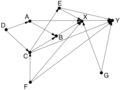
In fact, the full model in Forbes' paper has a few more variables and looks like the diagram in Figure 4.7. Note that Game 5 is embedded in this model in the sense that the variables A , B , C , X , and Y have exactly the same relationships. So we can transfer our conclusions over and conclude that we have to control for A and B or for C ; but C is an unobservable and therefore uncontrollable variable. In addition we have four new confounding variables: D = parental asthma, E = chronic bronchitis, F = sex, and G = socioeconomic status. The reader might enjoy figuring out that we must control for E F , , and G , but there is no need to control for D . So a sufficient set of variables for deconfounding is A B E F , , , , and G .
FIGURE 4.7. Andrew Forbes's model of smoking ( X ) and asthma ( Y ).
In the end, Forbes found that smoking had a small and statistically insignificant association with adult asthma in the raw data, and the effect became even smaller and more insignificant after adjusting for the confounders. The null result should not detract, however, from the fact that his paper is a model for the 'skillful interrogation of Nature.'
One final comment about these 'games': when you start identifying the variables as smoking, miscarriage, and so forth, they are quite obviously not games but serious business. I have referred to them as games because the joy of being able to solve them swiftly and meaningfully is akin to the pleasure a child feels on figuring out that he can crack puzzles that stumped him before.
Few moments in a scientific career are as satisfying as taking a problem that has puzzled and confused generations of predecessors and reducing it to a straightforward game or algorithm. I consider the complete solution of the confounding problem one of the main highlights of the Causal Revolution because it ended an era of confusion that has probably resulted in many wrong decisions in the past. It has been a quiet revolution, raging primarily in
research laboratories and scientific meetings. Yet, armed with these new tools and insights, the scientific community is now tackling harder problems, both theoretical and practical, as subsequent chapters will show.
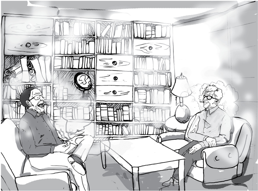
'Abe and Yak' (left and right, respectively) took opposite positions on the hazards of cigarette smoking. As was typical of the era, both were smokers (though Abe used a pipe). The smoking-cancer debate was unusually personal for many of the scientists who participated in it. ( Source: Drawing by Dakota Harr.)