Learning Cause-Effect Models
Readers who are familiar with the conditional statistical independence-based approach to causal discovery from observational data [Pearl, 2009, Spirtes et al., 2000] may be surprised by a chapter discussing causal inference for the case of only two observed variables, that is, a case where no non-trivial conditional independences can hold. This chapter introduces assumptions under which causal inference with just two observed variables is possible.
Some of these assumptions may seem too strong to be realistic, but one should keep in mind that empirical inference, even if it is not concerned with causal problems, requires strong assumptions. This is true in particular when it deals with high-dimensional data and low sample sizes. Therefore, oversimplified models are ubiquitous and they have been proven helpful in many learning scenarios.
The list of assumptions is diverse and we are certain that it is incomplete, too. Current research is still in a phase of exploring the enormous space of assumptions that yield identifiability between cause and effect. We hope that this chapter inspires the reader who may then add other - hopefully realistic - assumptions that can be used for learning causal structures.
We provide the assumptions and theoretical identifiability results in Section 4.1; Section 4.2 shows how these results can be used for structure identification in the case of a finite amount of data.
4.1 Structure Identifiability
4.1.1 Why Additional Assumptions Are Required
In Chapter 3, we introduced SCMs where the effect E is computed from the cause C using a function assignment. One may wonder whether this asymmetry of the data-generating process (i.e., that E is computed from C and not vice versa) becomes apparent from looking at P(C,E) alone. That is, does the joint distribution P(X,Y) of two variables X, Y tell us whether it has been induced by an SCM from X to Y or from Y to X? In other words, is the structure identifiable from the joint distribution? The following known result shows that the answer is 'no' if one allows for general SCMs.
Proposition 4.1 (Non-uniqueness of graph structures) For every joint distribution P(X,Y) of two real-valued variables, there is an SCM
$$Y = f_Y(X, N_Y), \quad X \perp N_Y,$$
where f_Y is a measurable function and N_Y is a real-valued noise variable.
Proof. Analogously to Peters [2012, Proof of Proposition 2.6], define the conditional cumulative distribution function
$$F_{Y|x}(y) := P(Y \leq y | X = x).$$
Then define
$$f_Y(x, n_Y) := F_{Y|x}^{-1}(n_Y),$$
where $F_{Y|x}^{-1}(n_Y) := \inf{x \in \mathbb{R} : F_{Y|x}(x) \geq n_Y}$. Then, let N_Y be uniformly distributed on [0,1] and independent of X. □
The result can be applied to the case X = C and Y = E as well as to the case X = E and Y = C, thus every joint distribution P(X,Y) admits SCMs in both directions. For this reason, it is often thought that the causal direction between just two observed variables cannot be inferred from passive observations alone. We will see in Chapter 7 that this claim fits into a framework in which causal inference is based on (conditional) statistical independences only [Spirtes et al., 2000, Pearl, 2009]. Then, the causal structures X → Y and Y → X are indistinguishable. For just two variables, the only possible (conditional) independence would condition on the empty set, which does not render X and Y independent unless the causal influence is non-generic. More recently, this perspective has been challenged by approaches that also use information about the joint distribution other than conditional independences. These approaches rely on additional assumptions about the relations between probability distributions and causality.
The remaining part of Section 4.1 discusses under which assumptions the graph structure can be recovered from the joint distribution (structure identifiability). Section 4.2 then describes methods that estimate the graph from a finite data set (structure identification). These statistical methods do not need to be motivated by the proofs of the identifiability results. Methods that follow the proofs closely are often inefficient in making use of the data.
4.1.2 Overview of the Type of Assumptions
A Priori Restriction of the Model Class One possible approach to distinguish cause and effect is to define a class of 'particularly natural' conditionals P(E|C) and marginals P(C). For several such classes, there are theoretical results showing that 'generic' combinations of marginals P(X) and conditionals P(Y|X) induce joint distributions that cannot be described by the same class when X and Y are swapped. Statements of this kind are also called identifiability results and we will see such examples in the remainder of Section 4.1.
For example, one may define classes of conditionals P(E|C) and marginals P(C) by restricting the class of functions f_E; see (3.2), and/or the class of noise distributions in (3.1) and (3.2), as will be discussed in Sections 4.1.3-4.1.6. This approach seems particularly natural from a machine learning perspective, where restricting the complexity of functions appears everywhere in standard tasks such as regression and classification. Note that inferring causal directions via restricted function classes implicitly assumes that the noise variables are still independent, in agreement with the definition of an SCM (see Definition 3.1). In this sense, one could say that these methods employ the independence of noise according to Figure 2.2, but keep in mind that independence of noise renders causal directions only identifiable after restricting the function class (see Proposition 4.1).
Another option of classes can be found in Sun et al. [2006], Janzing et al. [2009b], and Comley and Dowe [2003]. Sun et al. [2006] and Janzing et al. [2009b], for instance, consider second-order exponential models, for which the logarithmic densities of P(E|C) and P(C) are second order polynomials in e and c (up to a partition function), or in c, respectively.
We conclude this part with two questions: First, how should one define model classes that describe a reasonable fraction of empirical data in real life? Second, given that an empirical distribution admits such a model in exactly one direction, why should this be the causal one? The first question is actually not specific to the problem of causal inference; constructing functions that describe relations between observed variables always requires us to fit functions from a 'reasonable' class. The second question appears to be among the deepest problems concerning the relation between probability and causality. We are only able to give some intuitive and vague ideas, which now follow.
We start by providing an intuitive motivation that is related to the reason why usual machine learning relies on restricted model classes. Whenever we find a model from a small function class that fits our limited number of data, we expect that the model will also fit future observations, as argued in Chapter 1. Hence, finding models from a small class that fit data is crucial for the ability to generalize to future observations. Formally, learning causal models is substantially different from the usual learning scenario because it aims at inferring a model that describes the behavior of the system under interventions and not just observations taken from the same distribution. Therefore, there is no straightforward way to adopt arguments from statistical learning theory, to obtain a learning theory for causal relations. Nevertheless, we believe that finding a model from a small class suggests - up to some error probability - that the model will also hold under different background conditions. We further believe that models that hold under many different background conditions are more likely to be causal than models that just fit observations from a single data set (see 'Different Environments' in Section 7.1.6). This way, cause-effect inference via restricting the model class is vaguely related to ideas from statistical learning theory although drawing the exact link has to be left to the future. The preceding informal arguments for using causal models from small classes should not be mistaken as stating that causal relations in nature are indeed simple. The question whether or not we will often succeed in fitting data with simple functions, is a completely different question. We only argue for the belief that if there is a simple function that fits the data, it is more likely to also describe a causal relation. Furthermore, we will draw one connection between restricted model classes and the independence of cause and mechanism in Section 4.1.9. To be prepared for those quite formal derivations, we first provide a rather unrealistic toy model that we consider more a metaphor than a serious example.
Independence of Cause and Mechanism Section 2.1 describes the idea that P(C) and P(E|C) correspond to two independent mechanisms of nature. Therefore, they typically contain no information about each other (cf. Principle 2.1 and the middle box in Figure 2.2). Naturally, postulating that P(C) and P(E|C) are independent in the sense that they do not contain information about each other raises the question of what type of information is meant. There is no obvious sense in which the postulate can be formalized by a condition that could be checked by a statistical independence test. This is because we are talking about a scenario where one fixed joint distribution P(C,E) is visible and not a collection of distributions in which we could check whether the distribution of the hypothetical cause and the distribution of the hypothetical effect, given the cause, change in a dependent way (this is essentially the difference between the left and the middle boxes in Figure 2.2). To translate the independence of cause and mechanism into the language of SCMs, we assume that the distribution of the cause should be independent of the function and the noise distribution representing the causal mechanism. Note that this is, again, a priori, not a statement about statistical independence. Instead, it states that f_E and P(N_E) contain no information about P(C) and vice versa. This fact can only be used for causal inference if the independence is violated for all structural models that describe P(C,E) from E to C.
Sections 4.1.7 and 4.1.8 describe two toy scenarios for which well-defined notions of independence versus dependence can be given. Finally, in Section 4.1.9, we describe a formalization of independence of P(C) and P(E|C) that is applicable to more general scenarios rather than being restricted to the simple toy scenarios in Sections 4.1.7 and 4.1.8. Here, dependence is measured by means of algorithmic mutual information, a concept that is based on description length in the sense of Kolmogorov complexity. Since the latter is uncomputable, it should be considered as a philosophical principle rather than a method. Its practical relevance is two-fold. First, it may inspire the development of new methods and, second, justifications of existing methods can be based on it. For instance, the independence principle can justify inference methods based on an a priori restriction of the model class; see Section 4.1.9 for a specific example. To get a rough intuition about how independence is related to restricted model classes, consider a thought experiment where P(C) is randomly chosen from a class of k different marginal distributions. Likewise, assume that P(E|C) is chosen from another class of ℓ different conditional distributions. This induces k·ℓ different joint distributions P(C,E). In the generic case (unless the classes are defined in a rather special way), this yields k·ℓ > k different marginals P(E) and k·ℓ > ℓ different conditionals P(C|E). Hence, typical combinations of P(C) and P(E|C) induce joint distributions P(E,C) for which the 'backward marginal and conditional' P(E) and P(C|E) will not be in the original classes and would require larger model classes instead. In other words, no matter how large one chooses the set of possible P(C) and P(E|C), the set of induced P(C|E) and P(E) is even larger. This thought experiment is more like a metaphor because it is based on the naive picture of randomly choosing from a finite set. Nevertheless, it motivates the belief that in the causal direction, marginals and conditionals are more likely to admit a description from an a priori chosen small set provided that the latter has been constructed in a reasonable way.
Sections 4.1.3 to 4.1.6 describe model assumptions with a priori restriction of the model class, while Sections 4.1.7 to 4.1.9 formalize an independence assumption. Section 4.1.9, however, plays a special role because it should be considered a foundational principle rather than an inference method in its own right.
4.1.3 Linear Models with Non-Gaussian Additive Noise
While linear structural equations with Gaussian noise have been extensively studied, it has been observed more recently [Kano and Shimizu, 2003, Shimizu et al., 2006, Hoyer et al., 2008a] that linear non-Gaussian acyclic models (LiNGAMs) allow for new approaches to causal inference. In particular, the distinction between X causes Y and Y causes X from observational data becomes feasible. The assumption is that the effect E is a linear function of the cause C up to an additive noise term:
$$E = aC + N_E, \quad N_E \perp C,$$
with a ∈ ℝ (which is a special case of additive noise models introduced in Section 4.1.4). The following result shows that this assumption is sufficient for identifying cause and effect.
Theorem 4.2 (Identifiability of linear non-Gaussian models) Assume that P(X,Y) admits the linear model
$$Y = aX + N_Y, \quad N_Y \perp X, \quad (4.1)$$
with continuous random variables X, N_Y, and Y. Then there exist b ∈ ℝ and a random variable N_X such that
$$X = bY + N_X, \quad N_X \perp Y, \quad (4.2)$$
if and only if N_Y and X are Gaussian.
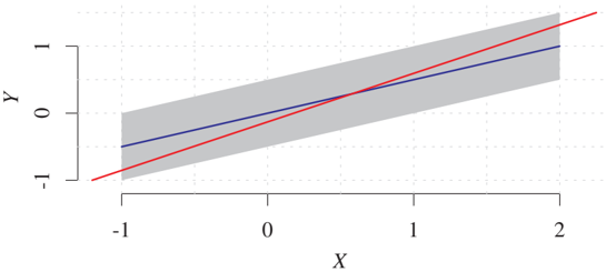
Figure 4.1: Joint density over X and Y for an identifiable example. The blue line is the function corresponding to the forward model Y := 0.5 · X + N_Y, with uniformly distributed X and N_Y; the gray area indicates the support of the density of (X,Y). Theorem 4.2 states that there cannot be any valid backward model since the distribution of (X,N_Y) is non-Gaussian. The red line characterized by (b,c) is the least square fit minimizing E[X - bY - c]². This is not a valid backward model X = bY + c + N_X since the resulting noise N_X would not be independent of Y (the size of the support of N_X would differ for different values of Y).
Hence, it is sufficient that C or N_E are non-Gaussian to render the causal direction identifiable; see Figure 4.1 for an example.
Let us look into slightly more details on how this result is proved. Theorem 4.2 is the bivariate case of the model class LiNGAM introduced by Shimizu et al. [2006], who prove a multivariate version of Theorem 4.2 using independent component analysis (ICA) [Comon, 1994, Theorem 11]. The proof of ICA is based on a characterization of the Gaussian distribution that was proved independently by Skitovič and Darmois [Skitovič, 1954, 1962, Darmois, 1953] and that we now state.
Theorem 4.3 (Darmois-Skitovič) Let X₁, ..., Xd be independent, non-degenerate random variables (see Appendix A.1). If there exist non-vanishing coefficients a₁, ..., ad and b₁, ..., bd (that is, for all i, aᵢ ≠ 0 ≠ bᵢ) such that the two linear combinations
$$l₁ = a₁X₁ + ... + adXd,$$ $$l₂ = b₁X₁ + ... + bdXd$$
are independent, then each Xᵢ is normally distributed.
It turns out that one can prove the bivariate version stated in Theorem 4.2 as a short and direct consequence from the theorem of Darmois-Skitovič; for illustration purposes we attach this proof in Appendix C.1. Furthermore, it can be shown that the identifiability of bivariate SCMs generalizes to identifiability of multivariate SCMs [Peters et al., 2011b]. With this result, the multivariate identifiability of LiNGAM then follows from Theorem 4.2.
Linear models with non-Gaussian additive noise can also be applied to a problem that sounds uncommon from the perspective of machine learning but that is interesting from the perspective of theoretical physics: estimating the arrow of time from data. Peters et al. [2009b] show that autoregressive models are time-reversible if and only if the noise variables are normally distributed. To explore asymmetries of empirical time series, they infer the time direction by fitting two autoregressive models, one from the past to the future, as standard, and one from the future to the past. In their experiments, the noise variables for the former direction indeed tend to be more independent than in the inverted time direction (cf. Section 4.2.1). Bauer et al. [2016] extend the idea to multivariate time series. Janzing [2010] links this observed asymmetry to the thermodynamic arrow of time, which suggests that asymmetries between cause and effect discussed in this book are also related to fundamental questions in statistical physics.
4.1.4 Nonlinear Additive Noise Models
We now describe additive noise models (ANMs), a less extreme restriction of the class of SCMs that is still strong enough to render cause-effect inference feasible.
Definition 4.4 (ANMs) The joint distribution P(X,Y) is said to admit an ANM from X to Y if there is a measurable function f_Y and a noise variable N_Y such that
$$Y = f_Y(X) + N_Y, \quad N_Y \perp X. \quad (4.3)$$
By overloading terminology, we say that P(Y|X) admits an ANM if (4.3) holds.
The following theorem shows that 'generically,' a distribution does not admit an ANM in both directions at the same time.
Theorem 4.5 (Identifiability of ANMs) For the purpose of this theorem, let us call the ANM (4.3) smooth if NY and X have strictly positive densities p{NY} and p_X, and f_Y, p{N_Y}, and p_X are three times differentiable.
Assume that P(Y|X) admits a smooth ANM from X to Y, and there exists a y ∈ ℝ such that
$$(\log p_{N_Y})''(y - f_Y(x)) f_Y'(x) ≠ 0 \quad (4.4)$$
for all but countably many values x. Then, the set of log densities log p_X for which the obtained joint distribution P(X,Y) admits a smooth ANM from Y to X is contained in a 3-dimensional affine space.
Proof. (Sketch of the idea. For details, see Hoyer et al. [2009]) The ANM from Y to X, given by
$$p(x,y) = p_Y(y) p_{N_X}(x - f_X(y)), \quad (4.5)$$
implies
$$\log p(x,y) = \log p_Y(y) + \log p_{N_X}(x - f_X(y)).$$
One can show that log p(x,y) then satisfies the following differential equation:
$$\frac{\partial}{\partial x}\left(\frac{\partial² \log p(x,y)/\partial x²}{\partial² \log p(x,y)/(\partial x \partial y)}\right) = 0. \quad (4.6)$$
On the other hand, the ANM from X to Y reads
$$p(x,y) = p_X(x) p_{N_Y}(y - f_Y(x)). \quad (4.7)$$
Taking the logarithm of (4.7) yields
$$\log p(x,y) = \log p_X(x) + \log p_{N_Y}(y - f_Y(x)). \quad (4.8)$$
Applying (4.6) to (4.8) yields a differential equation for the third derivative of log pX in terms of (first, second, and third) derivatives of f_X and log p{NY}. Thus, f_X and p{NE} (which are properties of the conditional P(Y|X)) determine log p_X up to the three free parameters log p{NX}(n), (log p{NX})'(n), and (log p{N_X})''(n) for an arbitrary point n. □
Theorem 4.5 states identifiability in the 'generic' case, where 'generic' is characterized by complicated conditions such as (4.4) and the three-dimensional subspace. For the case where pX and p{N_Y} is Gaussian, there is a much simpler identifiability statement saying that only linear functions f generate distributions that admit an ANM in backward direction [see Hoyer et al., 2009, Corollary 1]. Figure 4.2 visualizes two 'non-generic' examples of bivariate distributions that admit additive noise models in both directions. First, the obvious case of a bivariate Gaussian and, second, a sophisticated one that requires fine-tuning between p_X and N_X [Mooij et al., 2016].
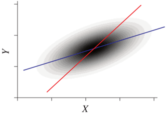
Figure 4.2: Joint density over X and Y for two non-identifiable examples. The left panel shows the linear Gaussian case and the right panel shows a slightly more complicated example, with 'fine-tuned' parameters for function, input, and noise distribution (the latter plot is based on kernel density estimation). The blue function f_Y corresponds to the forward model Y := f_Y(X) + N_Y, and the red function f_X to the backward model X := f_X(Y) + N_X.
To relate Theorem 4.5 to causal semantics, assume first that we know a priori that the joint distribution P(X,Y) of cause and effect admits an ANM from C to E, but we do not know whether X = C and Y = E or vice versa. Theorem 4.5 then states that generically there will not be an ANM from E to C, and we can thus easily decide which one of the variables is the cause C.
In general, however, conditionals P(E|C) in nature are not so strongly restricted that they necessarily admit an ANM. But is it possible that P(C) and P(E|C) then induce a joint distribution P(C,E) that admits an ANM from E to C? (In this case, we would infer the wrong causal direction.) We argue in Section 4.1.9 that this is unlikely if P(C) and P(E|C) are independently chosen.
4.1.5 Discrete Additive Noise Models
Additive noise can be defined not solely for real-valued variables, but for any variable that attains values in a ring. Peters et al. [2010, 2011a] introduce ANMs for the rings ℤ and ℤ/mℤ. That is, the set of integers and the set of integers modulo m ∈ ℤ. In the latter ring, we identify numbers that have the same remainder after division by m. For example, both integers 132 and 4 have the remainder (namely 4) after dividing by 8 and we write 132 ≡ 4 mod 8. Such a modular arithmetic may be appropriate when one of the domains inherits a cyclic structure. If we consider the day of the year, for example, we may want the days December 31 and January 1 to have the same distance as August 25 and August 26.
As in the continuous case, we can show that in the generic case, a joint distribution admits an ANM in at most one direction. The following result considers the example of the ring ℤ.
Theorem 4.6 (Identifiability of discrete ANMs) Assume that a distribution P(X,Y) allows for an ANM Y = f(X) + NY from X to Y and that either X or Y has finite support. P(X,Y) allows for an ANM from Y to X if and only if there exists a disjoint decomposition ⋃{i=0}^l C_i = supp X, such that the following conditions a), b), and c) are satisfied:
a) The C_i's are shifted versions of each other
$$∀i ∃ d_i ≥ 0: C_i = C_0 + d_i$$
and f is piecewise constant: f|_{C_i} ≡ c_i ∀ i.
b) The probability distributions on the C_i's are shifted and scaled versions of each other with the same shift constant as above: For x ∈ C_i, P(X = x) satisfies
$$P(X = x) = P(X = x - d_i) · \frac{P(X ∈ C_i)}{P(X ∈ C_0)}.$$
c) The sets c_i + supp N_Y := {c_i + h : P(N_Y = h) > 0} are disjoint sets.
(By symmetry, such a decomposition satisfying the same criteria also exists for the support of Y.) Figure 4.3 shows an example that allows an ANM in both directions [Peters et al., 2011a].
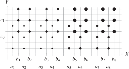
Figure 4.3: Only carefully chosen parameters allow ANMs in both directions (radii correspond to probability values); see Theorem 4.6. The sets described by the theorem are C₀ = {a₁, a₂, ..., a₈} and C₁ = {b₁, b₂, ..., b₈}. The function f takes the values c₀ and c₁ on C₀ and C₁, respectively.
There are similar results available for discrete ANMs modulo m. We refer to Peters et al. [2011a] for all details; we would like to mention, however, that the uniform noise distribution plays a special role: Y ≡ f(X) + N_Y mod m with a noise variable that is uniformly distributed on {0, ..., m-1} leads to independent X and Y and therefore allows an ANM from Y to X, too.
A discrete ANM imposes strong assumptions on the underlying process that are often violated in practice. As in the continuous case, we want to argue that if the process allows for a discrete ANM in one direction, it might be reasonable to infer that direction as causal (see also Section 4.1.9).
4.1.6 Post-nonlinear Models
A more general model class than the one presented in Section 4.1.4 has been analyzed by Zhang and Hyvärinen [2009]; see also Zhang and Chan [2006] for an early reference.
Definition 4.7 (Post-nonlinear models) The distribution P(X,Y) is said to admit a post-nonlinear model if there are functions f_Y, g_Y and a noise variable N_Y such that
$$Y = g_Y(f_Y(X) + N_Y), \quad N_Y \perp X. \quad (4.9)$$
The following result essentially shows that a post-nonlinear model exists at most in one direction except for some 'rare' non-generic cases.
Theorem 4.8 (Identifiability of post-nonlinear models) Let P(X,Y) admit a post-nonlinear model from X to Y as in (4.9) such that p_X, f_Y, g_Y are three-times differentiable. Then it admits a post-nonlinear model from Y to X only if p_X, f_Y, g_Y are adjusted to each other in the sense that they satisfy a differential equation described in Zhang and Hyvärinen [2009].
4.1.7 Information-Geometric Causal Inference
To provide an idea of how independence between P(E|C) and P(C) can be formalized, this section describes information-geometric causal inference (IGCI). IGCI, in particular the simple version described here, is a highly idealized toy scenario that nicely illustrates how independence in one direction implies dependence in the other direction [Daniušis et al., 2010, Janzing et al., 2012]. It relies on the (admittedly strong) assumption of a deterministic relation between X and Y in both directions; that is,
$$Y = f(X) \text{ and } X = f^{-1}(Y).$$
In other words, the noise variable in (3.2) is constant. Then the principle of independence of cause and mechanism described in Section 4.1.2 reduces to the independence of P(X) and f. Remarkably, this independence implies dependence between P(Y) and f^{-1}. To show this, we consider the following special case of the more general setting of Daniušis et al. [2010].
Definition 4.9 (IGCI model) Here, P(X,Y) is said to satisfy an IGCI model from X to Y if the following conditions hold: Y = f(X) for some diffeomorphism f of [0,1] that is strictly monotonic and satisfies f(0) = 0 and f(1) = 1. Moreover, P(X) has the strictly positive continuous density p_X, such that the following 'independence condition' holds:
$$\text{cov}[\log f', p_X] = 0, \quad (4.10)$$
where log f' and p_X are considered as random variables on the probability space [0,1] endowed with the uniform distribution.
Note that the covariance in (4.10) is explicitly given by
$$\text{cov}[\log f', p_X] = \int_0^1 \log f'(x) p_X(x) dx - \int_0^1 \log f'(x) dx \int_0^1 p_X(x) dx = \int_0^1 \log f'(x) p_X(x) dx - \int_0^1 \log f'(x) dx.$$
The following result is shown in Daniušis et al. [2010] and Janzing et al. [2012].
Theorem 4.10 (Identifiability of IGCI models) Assume the distribution P(X,Y) admits an IGCI model from X to Y. Then the inverse function f^{-1} satisfies
$$\text{cov}[\log (f^{-1})', p_Y] ≥ 0, \quad (4.11)$$
with equality if and only if f is the identity.
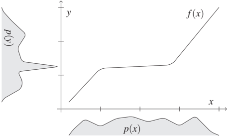
Figure 4.4: Visualization of the idea of IGCI: Peaks of p_Y tend to occur in regions where f has small slope and f^{-1} has large slope (provided that p_X has been chosen independently of f). Thus p_Y contains information about f^{-1}. IGCI can be generalized to non-differentiable functions f [Janzing et al., 2015].
In other words, uncorrelatedness of log f' and p_X implies positive correlation between log (f^{-1})' and p_Y except for the trivial case f = id. This is illustrated in Figure 4.4. It can be shown [Janzing and Schölkopf, 2015] that uncorrelatedness of f' and p_X (i.e., the analogue of (4.10) without logarithm) implies positive correlations between (f^{-1})' and p_Y, but IGCI uses logarithmic derivatives because this admits various information-theoretic interpretations [Janzing et al., 2012]. As justification of (4.10), Janzing et al. [2012] describe a model where f is randomly generated independently of P(X) and shows that (4.10) then holds approximately with high probability. It should be emphasized, however, that such justifications always refer to oversimplified models that are unlikely to describe realistic situations. Note that IGCI can easily be extended to bijective relations between vector-valued variables (as already described by Daniušis et al. [2010, Section 3]), but bijective deterministic relations are rare for empirical data. Therefore, IGCI only provides a toy scenario for which cause-effect inference is possible by virtue of an approximate independence assumption. The assumptions of IGCI have also been used [Janzing and Schölkopf, 2015] to explain why the performance of semi-supervised learning depends on the causal direction as stated in Section 5.1. By no means, is (4.10) meant to be the correct formalization of independence of cause and mechanism, nor do we believe that a unique formalization exists. Sgouritsa et al. [2015], for instance, propose an 'unsupervised inverse regression' technique that tries to predict P(Y|X) from P(X) and P(X|Y) from P(Y); they then suggest that the direction with the poorer performance is the causal one. Hence, this approach interprets 'independence' as making such kind of unsupervised prediction impossible.
4.1.8 Trace Method
Janzing et al. [2010] and Zscheischler et al. [2011] describe an IGCI-related independence between P(C) and P(E|C) for the case where C and E are high-dimensional variables coupled by a linear SCM:
Definition 4.11 (Trace condition) Let X and Y be variables with values in ℝᵈ and ℝᵉ, respectively, satisfying the linear model
$$Y = AX + N_X, \quad N_X \perp X, \quad (4.12)$$
where A is an e × d matrix of structure coefficients. Then P(X,Y) is said to satisfy the trace condition from X to Y if the covariance matrix S_{XX} and A are 'independent' in the sense that
$$t_e(AS_{XX}A^T) = t_d(S_{XX}) \cdot t_e(AA^T), \quad (4.13)$$
where t_k(B) := tr(B)/k denotes the renormalized trace of a matrix B.
A simple case that violates the trace condition would be given by a matrix A that shrinks all eigenvectors of S*{XX} corresponding to large eigenvalues and stretches those with small eigenvalues. This would certainly suggest that A has not been chosen independently of S*{XX}. Roughly speaking, (4.13) describes an uncorrelatedness between the eigenvalues of S*{XX} and the factor by which A changes the length of the corresponding eigenvectors. More formally, (4.13) can be justified by a generating model with large d, e, in which S*{XX} and A are independently chosen at random according to an appropriate (rotation invariant) prior probability. Then they satisfy (4.13) approximately with high probability [Besserve et al., in preparation]. For deterministic invertible relations, the causal direction is identifiable.
Theorem 4.12 (Identifiability via the trace condition) Let both variables X and Y be d-dimensional with Y = AX, where A is invertible. If the trace condition (4.13) from X to Y is fulfilled, then the backward model
$$X = A^{-1}Y$$
satisfies
$$t_d(A^{-1}S_{YY}A^{-T}) ≤ t_d(S_{YY}) \cdot t_d(A^{-1}A^{-T}),$$
with equality if and only if all singular values of A have the same absolute value.
Proof. The proof follows by applying Theorem 2 in Janzing et al. [2010] to the case n := m := d and observing that cov[Z, 1/Z] is negative whenever Z is a strictly positive random variable that is almost surely not constant. □
Hence, in the generic case, the trace condition is violated in backward direction and the violation of the equality has always the same sign.
For noisy relations, no statement like Theorem 4.12 is known. One can still check whether (4.13) approximately holds in one of the directions and infer this to be the causal one. Then the structure matrix for the causal model from Y to X is no longer given by A^{-1}. In this case, we introduce the notation A_X for the model from X to Y and A_Y for the model from Y to X. What makes the deterministic case particularly nice is the fact that the quotient
$$\frac{t(A_X S_{YY} A_X^T)}{t(A_X A_X^T) t(S_{YY})}$$
is known to be smaller than 1 because A_X = A_Y^{-1}.
The theoretical justification of independence conditions like (4.10), (4.13), and others mentioned in this book rely on highly idealized generating models (for instance, (4.13) has been justified by a model where the covariance matrix of the cause is generated from a rotation invariant prior [Janzing et al., 2010]). There is some hope, however, that violations of the idealized assumptions do not necessarily spoil the causal inference methods. The metaphor with the Beuchet chair may help to make this point. First, consider a scenario where the observational vantage point is chosen uniformly on a sphere. Clearly, this would contain no information about the orientation of the object. In this sense, the uniform prior formalizes an 'independence' assumption. Then the chair illusion only happens for a negligible fraction of angles. It is easy to see that strict uniformity for the choice of the vantage point is not needed to come to this conclusion. Instead, any random choice from a prior that is not concentrated within this small fraction of special angles will yield the same result. In other words, the conclusion about what a typical subject would see is robust with respect to violations of the underlying independence assumption. For this reason, discussions about the idealized assumptions of causal inference should focus on the question to what extent violations spoil the inference methods rather than explaining why they are too idealized.
4.1.9 Algorithmic Information Theory as Possible Foundation
This section describes an independence principle of which it is unclear how to apply it in practice although it relies on a well-defined mathematical formalism. It thus plays an intermediate role between the informal philosophical discussion about foundations of causal inference in Section 2.1 on the one hand and the concrete results of Sections 4.1.3 to 4.1.8 on possible asymmetries between cause and effect that rely on rather specific model assumptions on the other hand.
To formalize that P(E) and P(C|E) contain no information about each other for more general models than the ones considered in Sections 4.1.7 and 4.1.8 is challenging. It requires a notion of information that refers to objects other than random variables. This is because P(E) and P(C|E) are not random variables themselves but they describe distributions of random variables. One interesting notion of information is given by Kolmogorov complexity, which we briefly explain now.
Notions of Algorithmic Information Theory We first introduce Kolmogorov complexity: Consider a universal Turing machine T, that is, an abstraction of a computer that is ideal in the sense of having access to infinite memory space. For any binary string s, we define K_T(s) as the length of the shortest program, denoted by s*, for which T outputs s and then stops [Solomonoff, 1964, Kolmogorov, 1965, Chaitin, 1966, Li and Vitányi, 1997]. One may call s* the shortest compression of s, but keep in mind that s* contains all the information that T needs for running the decompression. Hence,
$$K_T(s) := |s*|,$$
where |·| denotes the number of digits of a binary word. This defines a probability-free notion of information content with respect to the given Turing machine T. In the following, we will refer to some fixed T and therefore drop the index. Although K(s) is uncomputable, that is, there is no algorithm that computes K(s) from s [Li and Vitányi, 1997], it can be useful to formalize conceptual ideas as it is done in this section.
The conditional algorithmic information of s, given t, is denoted by K(s|t) and defined as the length of the shortest program that generates the output s from the input string t and then stops. One can then define the mutual information as
$$I(s : t) := K(s) - K(s|t*).$$
In particular, we have [Chaitin, 1966]:
$$I(s : t) =^+ K(s) + K(t) - K(s,t), \quad (4.14)$$
where the symbol =^+ indicates that the equation only holds up to constants; that is, there is an error term whose length can be bounded independently of the lengths of s and t. To define Kolmogorov complexity K(s,t) for the pair (s,t), one constructs a simple bijection between strings and pairs of strings by first using some enumeration of strings and then using a standard bijection between ℕ and ℕ × ℕ.
A simple interpretation of (4.14) is that algorithmic mutual information thus quantifies the amount of memory space saved when compressing s, t jointly instead of compressing them independently. Janzing and Schölkopf [2010] argue that two objects whose binary descriptions s, t have a significant amount of mutual information are likely to be causally related. In other words, in the same way as statistical dependences between random variables indicate causal relations (see Principle 1.1), algorithmic dependences between objects indicate causal relations between objects. Observing, for instance, two T-shirts with similar designs produced by different companies may indicate that one company copied from the other. Indeed, similarity of patterns in real life may be described by algorithmic mutual information provided that one has first agreed on an 'appropriate' way to encode the pattern into a binary word and then on an 'appropriate' Turing machine. For the difficult question of what 'appropriate' means, see also the brief discussion of 'relative causality' in the introduction of Janzing et al. [2016].
Algorithmic Independence of Conditionals The principle of algorithmically independent conditionals has been stated by Janzing and Schölkopf [2010] and Lemeire and Janzing [2013] for multivariate causal structures, but it yields nontrivial implications already for the bivariate case.
For two variables C and E being cause and effect, we assume that P(C) and P(E|C) admit finite descriptions by binary strings s and t, respectively. In a parametric setting, s and t may describe points in the corresponding parameter spaces. Alternatively, one may think of s and t as being programs that compute p(c) and p(e|c) for all values c, e having finite description length. Then we use I(P(C) : P(E|C)) for I(s : t) and postulate:
Principle 4.13 (Algorithmically independent conditionals) P(C) and P(E|C) are algorithmically independent, that is,
$$I(P(C) : P(E|C)) =^+ 0, \quad (4.15)$$
or, equivalently,
$$K(P(C), P(E|C)) =^+ K(P(C)) + K(P(E|C)). \quad (4.16)$$
The equivalence of (4.15) and (4.16) is immediate because describing the pair (P(C), P(E|C)) is equivalent to describing the joint P(C,E). The idea of Principle 4.13 is that P(C) and P(E|C) are causally unrelated objects of nature. This is certainly an idealized assumption, but for a setting where X causes Y or Y causes X it suggests to infer X → Y whenever the algorithmic dependences between P(X) and P(Y|X) are weaker than for P(X|Y) and P(Y). To apply this to empirical data, however, raises the problem that P(X,Y) cannot be determined from finite data on top of the problem that algorithmic mutual information is uncomputable.
Despite these issues, Principle 4.13 is helpful to justify practical causal inference methods as we describe now for the example of ANMs. Janzing and Steudel [2010] argue that the SCM Y := f_Y(X) + N_Y implies that the second derivative of y ↦ log p(y) is determined by partial derivatives of (x,y) ↦ log p(x,y). Hence, knowing P(X|Y) admits a short description of P(Y) (up to some accuracy). Whenever K(P(Y)) is larger than this small amount of information, Janzing and Steudel [2010] conclude that Y → X should be rejected because P(Y) and P(X|Y) are algorithmically dependent. For any given data set we cannot guarantee that K(P(Y)) is large enough to reject Y → X just because there is an ANM from Y to X. However, when applying inference that is based on the principle of ANMs to a large set of different distributions, we know that most of the distributions P(Y) are complex enough (since the set of distributions with low complexity is small) to justify rejecting causal models that induce ANMs in the opposite direction. Moreover, Figure 5.4, left and right, shows two simple toy examples where looking at P(X) alone suggests a simple guess for the joint distribution P(X,Y). Indeed, one can show that this amounts to algorithmic dependence between P(X) and P(Y|X), as shown for the left case by Janzing and Schölkopf [2010, remarks after Equation (27)].
We should also point out that (4.15) implies
$$K(P(C)) + K(P(E|C)) =^+ K(P(C,E)) ≤ K(P(E)) + K(P(C|E)). \quad (4.17)$$
The equality follows because describing P(C,E) is equivalent to describing the pair (P(C), P(E|C)), which is not shorter than describing marginal and conditional separately. The inequality follows because P(E) and P(C|E) also determine P(C,E). In other words, independence of conditionals implies that the joint distribution has a shorter description in the causal direction than in the anticausal direction.
This implication also sounds natural from the perspective of the minimum description length principle [Grünwald, 2007] and in the spirit of Occam's razor.
Note, however, that the condition K(P(C)) + K(P(E|C)) ≤^+ K(P(E)) + K(P(C|E)) is strictly weaker than (4.15) since the shortest description of P(C,E) may not use either of the two possible factorizations, which can happen, for instance, when there is a hidden common cause [Janzing and Schölkopf, 2010, p. 16].
Principle 6.53 generalizes Principle 4.13 to the multivariate setting.
4.2 Methods for Structure Identification
We now present different ideas about how the identifiability results obtained in Section 4.1 can be exploited for causal discovery. That is, the methods estimate a graph from a finite data set. These are challenging statistical problems, which can be approached in many different ways. We try to focus on methodological ideas and do not claim that the methods we present make the most efficient use of the data. It is very well possible that future research will yield novel and successful methods. We restrict the attention to a few examples, mainly to those for which we have reasonable experience regarding their performance.
4.2.1 Additive Noise Models
For causal learning methods based on the identifiability of ANMs according to Theorem 4.5, we mainly refer to the multivariate chapter (Section 7.2). Here, we sketch two methods without claiming their optimality. The first method tests the independence of residuals and is a special case of the regression with subsequent independence test (RESIT) algorithm (see Section 7.2).
- Regress Y on X; that is, use some regression technique to write Y as a function f̂_Y of X plus some noise.
- Test whether Y - f̂_Y(X) is independent of X.
- Repeat the procedure with exchanging the roles of X and Y.
- If the independence is accepted for one direction and rejected for the other, infer the former one as the causal direction.
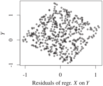
Figure 4.5: We are given a sample from the underlying distribution and perform a linear regression in the directions X → Y (left) and Y → X (right). The fitted functions are shown in the top row, the corresponding residuals are shown in the bottom row. Only the direction X → Y yields independent residuals; see also Figure 4.1.
Figure 4.5 shows the procedure on a simulated data set; see Figure 4.1 for the underlying distribution. At least in the continuous setting, the first two steps are standard problems of machine learning and statistics (see Appendices A.1 and A.2), with the additional challenge that they are coupled: f̂_Y deviating from f_Y may hide or create dependences between noise and input variable. In general, any test based on the estimated residuals may lose its type I error control. As a possible solution one may use sample splitting [Kpotufe et al., 2014]. Moreover, it is important to choose an independence test that accounts for higher order statistics rather than testing correlations only. Any regression technique minimizing quadratic error that includes linear components and an intercept yields uncorrelated noise. In practice, one may use the Hilbert-Schmidt Independence Criterion (HSIC) [Gretton et al., 2008], for example, which we briefly introduce in Appendix A.2. Mooij et al. [2016, Theorem 20] use a continuity property of HSIC to show that even without sample splitting, one obtains the correct value of HSIC in the limit of infinite data (there are no claims about the p-values of the test, however). Finally, the last step deserves our particular attention because it refers to the relation between probability and causality. Depending on the significance levels for rejecting and accepting independence, one may get an ANM in both directions, in no direction, or in one direction. To enforce decisions, one just infers the direction to be the causal one, for which the p-value for rejecting independence is higher.
Recent studies provide some evidence that this procedure yields success rates on real data above chance level [Mooij et al., 2016]. Figure 4.6 shows the scatter plot of real-world data for which an ANM holds reasonably well only in the causal direction. For modifications regarding discrete data, we refer to the corresponding literature [Peters et al., 2011a]. Note that the post-nonlinear model (4.9) is considerably harder to fit in practice than the more standard nonlinear regression model (4.3).
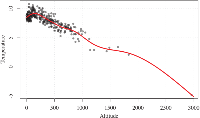
Figure 4.6: Relation between average temperature in degrees Celsius (Y) and altitude in meters (X) of places in Germany. The data are taken from 'Deutscher Wetterdienst,' see also Mooij et al. [2016]. A nonlinear function (which is close to linear in the regime far away from sea level) with additive noise fits these empirical observations reasonably well.
As an alternative to the preceding approach, one may also use a maximum likelihood-based approach. Consider a nonlinear SCM with additive Gaussian error terms, for example. One may then distinguish between X → Y and X ← Y by comparing the likelihood scores of both models. To do so, we first perform a nonlinear regression from Y on X to obtain residuals R_Y := Y - f̂_Y(X). We then compare
$$L_{X→Y} = -\log\text{var}[X] - \log\text{var}[R_Y] \quad (4.18)$$
with the analogous version
$$L_{X←Y} = -\log\text{var}[R_X] - \log\text{var}[Y] \quad (4.19)$$
that we obtain when interchanging the roles of X and Y. It is not difficult to show (see Problem 4.16) that this indeed corresponds to a comparison of likelihoods when instead of performing the regression, we use the true conditional mean f̂_Y(x) = E[Y|X = x] (and similarly for f̂_X). As before, however, this two-step procedure of first performing regression and then computing sample variances requires justification. Bühlmann et al. [2014] use empirical process theory [van de Geer, 2009] to prove consistency. If the noise does not necessarily follow a Gaussian distribution, we have to adapt the score functions by replacing the logarithm of the empirical variance of the residuals with an estimate of the differential entropy of the error term [Nowzohour and Bühlmann, 2016].
Code Snippet 4.14 The following code shows an example with a finite data set. It makes use of the code packages dHSIC [Pfister et al., 2017] and mgcv [Wood, 2006]. The former package contains the function dhsic.test, an implementation of the independence test proposed by [Gretton et al., 2008], and the latter package contains the function gam that we use as a nonlinear regression method in lines 10 and 11 (see Section A.1). Only in the backward direction is the independence between residuals and input rejected, see lines 15 and 17. In lines 21 and 23, we see that a Gaussian likelihood score favors the forward direction, too; see also Equations (4.18) and (4.19).
library(dHSIC)
library(mgcv)
#
# generate data set
set.seed(1)
X <- rnorm(200)
Y <- X^3 + rnorm(200)
#
# fit models
modelforw <- gam(Y ~ s(X))
modelbackw <- gam(X ~ s(Y))
#
# independence tests
dhsic.test(modelforw$residuals, X)$p.value
# [1] 0.7628932
dhsic.test(modelbackw$residuals, Y)$p.value
# [1] 0.004221031
#
# computing likelihoods
-log(var(X)) - log(var(modelforw$residuals))
# [1] 0.1420063
-log(var(modelbackw$residuals)) - log(var(Y))
# [1] -1.014013
4.2.2 Information-Geometric Causal Inference
We sketch the implementation of IGCI briefly and refer to Mooij et al. [2016] for details. The theoretical basis is given by the identifiability result in Theorem 4.10 and some simple conclusions thereof. One can show that the independence condition (4.10) implies
$$C_{X→Y} ≤ C_{Y→X}$$
if one defines
$$C_{X→Y} := \int_0^1 \log f'(x) p(x) dx,$$
and C_{Y→X} similarly. Here, the following straightforward estimators are used:
$$\hat{C}{X→Y} := \frac{1}{N-1} \sum{j=1}^{N-1} \log\frac{|y_{j+1} - y_j|}{|x_{j+1} - x_j|},$$
where the x₁ < x₂ < ··· < xN are the observed x-values in increasing order. If Y is an increasing function of X, the y-values are also ordered, but for real data this will usually not be the case. The estimator Ĉ{Y→X} is defined accordingly and X → Y is inferred whenever Ĉ*{X→Y} < Ĉ*{Y→X}. Apart from the so-called slope-based approach, there is also an entropy-based approach. One can show that (4.10) also implies
$$H(X) ≤ H(Y),$$
where H denotes the differential Shannon entropy
$$H(X) := -\int_0^1 p(x) \log p(x) dx.$$
Intuitively, the reason is that applying a nonlinear function f to p_X generates additional irregularities (unless the nonlinearity of f is tuned relative to p_X) and thus makes p_Y even less uniform than p_X. Accordingly, the variable with the larger entropy is assumed to be the cause. To estimate H, one can use any standard entropy estimator from the literature.
4.2.3 Trace Method
Recall that this method relies on linear relations between high-dimensional variables X and Y. First assume that the sample size is sufficiently large (compared to the dimensions of X and Y) to estimate the covariance matrices S*{XX} and S*{YY} and the structure matrices A_Y and A_X by standard linear regression. To employ the identifiability result in Theorem 4.12, one can compute the tracial dependency ratio
$$r_{X→Y} := \frac{t(A_Y S_{XX} A_Y^T)}{t(A_Y A_Y^T) t(S_{XX})},$$
and likewise r_{Y→X} (via swapping the roles of X and Y) and infer that the one that is closer to 1 corresponds to the causal direction [Janzing et al., 2010].
Zscheischler et al. [2011] describe a method to assess whether the deviation from 1 is significant, subject to a generating model where independence of the two matrices A and S*{XX} is simulated by some random orthogonal map rotating them against each other. Using ideas from free probability theory [Voiculescu, 1997], a mathematical framework that describes asymptotic behavior of large random matrices, Zscheischler et al. [2011] construct an implementation of the trace condition for the regime where the dimension is larger than the sample size. They show that, in the noiseless case, r*{X→Y} can still be estimated (although there is not enough data to estimate S*{XX} and A) subject to an additional independence assumption for A and the empirical covariance matrix of X. Therefore, one can reject the hypothesis X → Y whenever the estimator deviates significantly from 1. Then, either the additional independence assumption is wrong or r*{X→Y} deviates significantly from 1.
4.2.4 Supervised Learning Methods
Finally, we describe a method that approaches causal learning from a more machine learning point of view. It has, in principle, the ability to make use of either restricted function classes or an independence condition. Suppose, we are given labeled training data of the form (D₁, A₁), ..., (D_n, A_n). Here, each D_i is a data set
$$D_i = {(X₁, Y₁), ..., (X_{n_i}, Y_{n_i})}$$
containing realizations (X₁, Y₁), ..., (X*{n_i}, Y*{n_i}) i.i.d. ~ P_i(X,Y), and each label A_i ∈ {→, ←}, describes whether data set D_i corresponds to X → Y or X ← Y. Then, causal learning becomes a classical prediction problem, and one may train classifiers hoping that they generalize well from the data set with known ground-truth to unseen test data sets.
To the best of our knowledge, Guyon [2013] was the first one who systematically investigated such an approach in the form of a challenge (providing a mix of synthetic and real data sets as known ground truth data). It is clear that the method will not succeed by exploiting symmetric features as correlation or covariance.
Many of the competitive classifiers in the challenge were based on hand-crafted features; examples include entropy estimates of the marginal distributions or entropy estimates of the distribution of the residuals that resulted from regressing either X on Y or Y from X. Interestingly, such features can be related to the concept of ANMs. For Gaussian distributed variables, for example, the entropy is a linear function of the logarithm of the variance and, therefore, the features are expressive enough to reconstruct the scores (4.18) and (4.19). Considering entropies instead of logarithm of variances corresponds to relaxing the Gaussianity assumption [Nowzohour and Bühlmann, 2016].
López-Paz et al. [2015] aims at an automatic construction of such features. The idea is to map the joint distributions P_i(X,Y), i = 1, ..., n into a reproducing kernel Hilbert space (see Appendix A.2) and perform a classification in this space. In practice, one does not have access to the full distribution P_i(X,Y) and rather uses the empirical distribution as an approximation. (A similar approach has been used to distinguish time series that are reversed in time from their original version [Peters et al., 2009a].) Because the classification into cause and effect seems to rely on relatively complex properties of the joint distribution, one requires a large sample size n for the training set. To add useful simulated data sets, these must be generated from identifiable cases. López-Paz et al. [2015] use additional samples from ANMs, for example.
Supervised learning methods do not yet work as stand-alone methods for causal learning. They may prove to be useful, however, as statistical tools that can make efficient use of known identifiability properties or combinations of those.
4.3 Problems
Problem 4.15 (ANMs) a) Consider the SCM
$$X := N_X, \quad Y := 2X + N_Y$$
with N_X uniformly distributed between 1 and 3 and N_Y uniformly distributed between -0.5 and 0.5 and independent of N_X. The distribution P(X,Y) admits an ANM from X to Y. Draw the support of the joint distribution of X, Y and convince yourself that P(X,Y) does not admit an ANM from Y to X, that is there is no function g and independent noise variables M_X and M_Y such that
$$X = g(Y) + M_X, \quad Y = M_Y$$
with M_X independent of M_Y.
b) Similarly as in part a), consider the SCM
$$X := N_X, \quad Y := X² + N_Y$$
with N_X uniformly distributed between 1 and 3 and N_Y uniformly distributed between -0.5 and 0.5 and independent of N_X. Again, draw the support of P(X,Y) and convince yourself that there is no ANM from Y to X.
Problem 4.16 (Maximum likelihood) Assume that we are given an i.i.d. data set (X₁, Y₁), ..., (X_n, Y_n) from the model
$$Y = f(X) + N_Y, \quad \text{with } X \sim N(m_X, σ_X²), \text{ and } N_Y \sim N(m_{N_Y}, σ_{N_Y}²) \text{ independent,}$$
where the function f is supposed to be known.
a) Prove that f(x) = E[Y|X = x].
b) Write x := (x₁, ..., x_n), y := (y₁, ..., y_n) and consider the log-likelihood function
$$ℓ_q(x,y) = ℓ_q((x₁,y₁), ..., (x_n,y_n)) = \sum_{i=1}^n \log p_q(x_i, y_i),$$
where pq is the joint density over (X,Y) and q := (m_X, m{NY}, σ_X², σ{N_Y}²). Prove that for some c₁, c₂ ∈ ℝ with c₂ > 0
$$\max_q ℓ_q(x,y) = c₂ · (c₁ - \log\text{var}[x] - \log\text{var}[y - f(x)]), \quad (4.20)$$
where var[z] := (1/n)∑ᵢ₌₁ⁿ(z_i - (1/n)∑ₖ₌₁ⁿz_k)² estimates the variance.
Equation (4.20) motivates the comparison of expressions (4.18) and (4.19). The main difference is that in this exercise, we have used the conditional mean and not the outcome of the regression method. One can show that, asymptotically, the latter still produces correct results [Bühlmann et al., 2014].